That looks fine if you’re trying to achieve a straightforward boxfilter, but I think it’s 1D (therefore can’t be per-pixel window sizes) and handles portion boundaries by overlapping/extending them. Recursive boxfilter is what we have in g’mic already! As you say though, the main problem there is it’s unlikely to run in acceptable time inside the g’mic math interpreter vs compiled on gpu.
The problem with these methods is that they are so abstracted that they are inflexible. E.g., I wouldn’t know where to begin when it comes to addressing boundary conditions. Speaking of which, I have two questions about corners.
– Is your discussion on bi-linear interpolation about that?
– What does mirror do around the corners?
The bilinear is purely to handle non-integer window sizes. It should still function for locations outside the boundary (“virtual pixels”).
A quick way to visualise boundary handling in g’mic is using crop (shortcut = z):
gmic sp r2dx 200 m "foo: z -100%,-100%,200%,200%,$""1" +foo 0 +foo.. 1 +foo... 2 +foo[0] 3
Ha ha, I was staring at the spreadsheet and forgot to check in G’MIC. Looks like the corner is a mirror of a mirror, which is simpler than my conception of it being a diagonal mirror.
Just for fun, I have created IM process module “deintegim2”, which modulates the widow width and height according to the red and green channels of a map image.
So the window dimensions are controllable, in both directions. For simplicity and speed, calculated window dimensions are rounded to integers.
For example, we increase the window width in the horizontal direction across the image, and the window height in the vertical direction down the image, so the result is not blurred at top-left, blurred horizontally at top-right, blurred vertically bottom-left, and blurred in both directions bottom-right.
convert ^
  %SRC% ^
  -process integim ^
  ( +clone ^
    -sparse-color Bilinear ^
0,0,#000,^
%%[fx:w-1],0,#f00,^
0,%%[fx:h-1],#0f0,^
%%[fx:w-1],%%[fx:h-1],#ff0 ^
    -evaluate Pow 3 ^
  ) ^
  -process 'deintegim2 window 50x50' ^
  x.jpg

The effect is similar to IM’s built-in “-compose Blur … -composite”, which uses high-quality but computation-heavy Gaussian weighting, with Elliptical Weighted Averages. The IM window size is really the “sigma” for the linear Gaussian distribution.
convert ^
  %SRC% ^
  ( +clone ^
    -sparse-color Bilinear ^
0,0,#000,^
%%[fx:w-1],0,#f00,^
0,%%[fx:h-1],#0f0,^
%%[fx:w-1],%%[fx:h-1],#ff0 ^
    -evaluate Pow 3 ^
  ) ^
  -compose Blur ^
  -set option:compose:args 20x20 -composite ^
  x1.jpg

For small images and small windows, the performance of either method is fine.
For a 4924x7378 pixel image, with windows four times the linear dimensions (ie 200x200 and 80x80), my method is a factor of 188 faster than IM’s “-compose Blur … -composite” (68 seconds versus 12841 seconds).
Do we get to try this out ourselves? 
I’ve been thinking about doing a cimg/g’mic plugin to compare compiled speed, but I’ll likely never get around to it.
Interested by doing this in G’MIC. Will give a try.
Here is my attempt, with G’MIC.
The command foo below does the same kind of box blurring with box sizes that increases horizontally and vertically along the X and Y axes.
# $1 = min radius, $2 = max radius.
foo : skip ${1=1},${2=max(w,h)/10}
  repeat $! l[$>]
    100%,100%,1,2,"round([ lerp($1,$2,(x/w)^3), lerp($1,$2,(y/h)^3) ])"
    +cumulate[0] xy
    f[0] "*
      const W = w - 1; const H = h - 1;
      px(X,Y) = I(#2,X,Y,0,c);
      T(X,Y)=Y>1?px(X,Y-1):Y*px(X,0);
      B(X,Y)=Y<H?px(X,Y):(1+Y-H)*px(X,H)-(Y-H)*px(X,H-1);
      G(X,Y)=X<W?B(X,Y):(1+X-W)*B(W,Y)-(X-W)*B(W-1,Y);
      D(X,Y)=X>1?T(X-1,Y):X*T(0,Y);
      E(X,Y)=X<W?T(X,Y):(1+X-W)*T(W,Y)-(X-W)*T(W-1,Y);
      F(X,Y)=X>1?B(X-1,Y):X*B(0,Y);

      bw = i(#1,x,y,0,0);                     # Horizontal size of blur window
      bh = i(#1,x,y,0,1);                     # Vertical size of blur window
      bw1 = int(bw/2); bh1 = int(bh/2);       # Left/Top half-sizes
      bw0 = bw - bw1 - 1; bh0 = bh - bh1 - 1; # Right/Bottom half-sizes
      x0 = x - bw0;
      y0 = y - bh0;
      x1 = x + bw1;
      y1 = y + bh1;
      (G(x1,y1) + D(x0,y0) - E(x1,y0) - F(x0,y1))/(bw*bh)"
    k[0]
  endl done
It can be used like this:
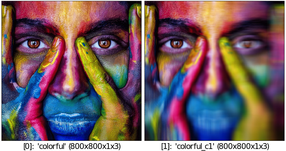
$ gmic sp colorful tic +foo , toc
[gmic]-0./ Start G'MIC interpreter.
[gmic]-1./ Input sample image 'colorful' (1 image 800x800x1x3).
[gmic]-1./ Initialize timer.
[gmic]-2./ Elapsed time: 0.093 s.
For a large image (8000x8000) :
$ gmic sp colorful,8000 tic +foo , toc
[gmic]-0./ Start G'MIC interpreter.
[gmic]-1./ Input sample image 'colorful' (1 image 8000x8000x1x3).
[gmic]-1./ Initialize timer.
[gmic]-2./ Elapsed time: 8.538 s.
[gmic]-2./ Display images [0,1] = 'colorful, colorful_c1'.
Timings look quite good to me.
EDIT : edited to better manage boundary conditions (by extending the image with Neumann conditions before processing).
EDIT2: Used @garagecoder trick to manage boundary conditions of SAT. Very efficient stuff !
1 Like
In case you missed this from earlier, I added a g’mic github wiki page about how I’ve done the Neumann boundary without extending the image.
You obviously have a nice machine there, even the first version took 38s on mine! I deliberately use a very old core2 for filter writing so I get a feel for “real world” usage though…
1 Like
Ah sorry, I’ve missed that indeed.
I’ll check and try to make a better version with your boundary tricks!
1 Like
deintegim2 is just a quick hack to answer the question: what is the quality and performance from a very simple implementation of window sizes driven by an image, with integer window sizes?
My conclusion is: quality and performance are acceptable.
Next question: what is the change in quality and performance for non-integer window sizes, using four-point lerf at each window corner?
I find it hard to see any benefit of fractional window sizes if all we need is a blurred image. I think that only becomes significant when used as a portion of some other filter. Something involving local gradients or variance perhaps? It’s difficult to predict… I like to include it just for completeness (it’s easier to remove it than add).
Performance wise, quite a large hit when done “manually” in a 64bit gmic buffer but probably not too terrible when compiled.
Tested your command on an 8K tiger. Takes about 1 min.
gmic sp tiger,8000 +f 1 tic +gcd_boxfilter_local.. . toc rm.. -
In terms of gcd_boxfilter_local_hp, it stops working at 8K with the error ouput
*** Error in ./gcd_boxfilter_local_hp/*repeat/*local/ *** Command 'fill': [instance(0,0,0,0,0000000000000000,non-shared)] gmic<double>::assign(): Failed to allocate memory (31.9 Gio) for image (4283106549,1,1,1).
I tried 4K but it stops without an error !
May need debugging.
With 4k I get this error:
[gmic] G'MIC encountered a fatal error. Please submit a bug report, at: https://github.com/dtschump/gmic/issues
On my Mac 8k shows the same fatal error, not with 4k!
Using gcd_boxfilter_local (or afre_box0):
gmic sp tiger / {iM} +sqr repeat 2 l[$>] +f 3 gcd_boxfilter_local.. . rm. endl done
min = 0.0112847     max = 1.00174
min = -0.000434028  max = 1.00087
Using gcd_boxfilter_local_hp:
min = 0.0120968     max = 1
min = 0.000146329   max = 1
In the first case, the outputs of the command aren’t within the domain of the input: lower mins and higher maxes. (Means don’t appear to be affected, at least not in this example.)
Yup, side effect of the limited precision. I don’t like to “hide” the error with a cut because that might not fit every scenario. Perhaps I’ll add a second parameter for cut/normalise/nothing. In the meantime, better to either wrap it inside another command or just plain copy the code and amend (or just do a cut on each use where needed).
Yes, strange, it looks like a link, but it actually links to nothing.
Sorry, doubled the parentheses by mistake, which preserved the formatting but dropped the link. Have fun with the integral histogram paper.