Hello folks,
I’ve added a new command in the standard library of G’MIC 2.9.1, and I think this could interest some of the G’MIC script writers here. I’m pretty sure this could lead to fun experimentations 
Release of stable G’MIC 2.9.1 is planed for tomorrow.
The new command is named rbf, which stands for Radial Basis Function. More precisely, it implements a RBF-based interpolation of sparse keypoints. To be honest, I’ve already been using RBF-interpolation in some of the G’MIC filters for a long time (commands x_warp, x_morph and clut, to name a few), but I’ve decided it was time to provide this generic interpolation method as a stand-alone command that can be used to interpolate any kind of data.
It basically works like this: the command takes as input a set of K keypoints (X_k,V_k) (where k=1\dots K). The X_k represents the coordinates of keypoint k (X_k can be a 1D/2D or 3D vector), and V_k is the associated value of keypoint k (V_k can be a N-dimensional vector, with N having any value). The set of keypoints is passed to rbf as a single-column (or single-row) vector-valued image, where each pixel represents a keypoint.
From this, the command rbf is able to interpolate the values of the keypoints in all 1D/2D or 3D image space. You specify the size of the interpolated image you want as a result, as well as a corresponding XYZ coordinate mapping (optionally).
To sum up, rbf creates a smooth function that passes through given keypoints.
Beware, if the number of keypoints increases, then processing time explodes. Even if the command is parallelized, it implies a K\times K matrix inversion (K, the number of keypoints), which usually has a complexity of O(K^3) + it has a reconstruction phase with complexity O(whdK). But if the set of keypoints is small enough (I’d say <1000), then it’s a very interesting toy to play with.
A few examples:
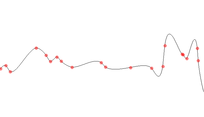
- 1D interpolation:
test1d :
  20,1,1,2,[u(700),u(150,250)]  # Pick random keypoints
  +rbf. 700                     # Interpolate keypoints
  700,400,1,3,255 round. graph. ..,1,0,0,400
  eval[0] "ellipse(#-1,i0,i1,5,5,0,0.5,255,0,0); I"
test1d gives:
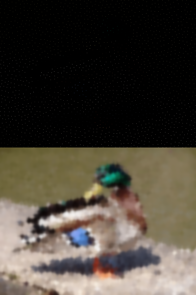
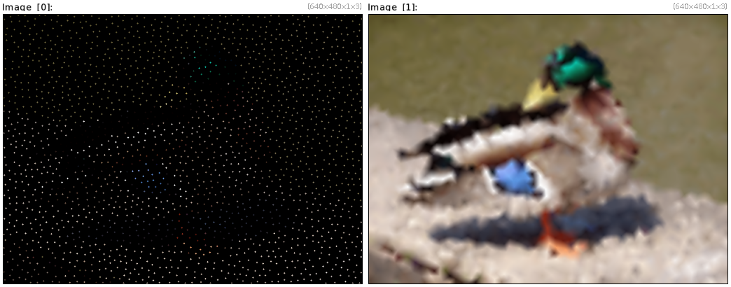
- 2D interpolation:
test2d :
  sp duck
  100%,100% noise_poissondisk. 10  # Pick random keypoints
  1,{is},1,5 eval[-2] "begin(p=0);i?(I[#-1,p++]=[x,y,I(#0)])" # Create set of 2D colored keypoints
  to_rgb[1] mul[0,1] dilate_circ[0] 5
  +rbf[-1] {0,[w,h]} c[-1] 0,255 rm..
test2d gives (after heating your CPUs a lot…):

-
Easy color gradient:
You can userbfto create super-easy random color gradients:
test2d_2 :
  32,1,1,5,u([400,400,255,255,255])
  rbf 400,400 c 0,255
test2d_2 gives:

That’s it. I’d be interested by what you can obtain with this new command.
Note that we already had solidify and inpaint_pde for doing such interpolation, but having another option is still cool.