Great article! Thanks @anon41087856, it makes much more easy for me as an end user (i.e. not DT developer) to understand the philosophy of the whole pixelpipe, and the place of each module on it.
I specially appreciate the sections on minimal workflow and replacement modules. I’m a light user of DT (not many pictures, so no constant use), and having a consistent and small base workflow helps me to focus and not having to re-learn which module to use for what every time I sit on the computer.
One correction: you talk several times about the “energy” of the light, when in fact you are referring to its “intensity”. Physically, the energy of the light is related to its wavelength (color), what’s proportional to the number of photons is its intensity. If I’m not mistaken, every single use of the word energy in the article is about that, so it should be an easy “replace energy → intensity”. Sorry, my physics background makes me cringe every time I read it
I agree that the energy of a photon is related to its wavelength. Is that what the article is discussing? Or is it the energy of the light (more than one photon), which is related to the number of photons? If one photon has energy E then n photons of the same wavelength have energy nE.
“Intensity” is probably a good substitution but I don’t know that it’s necessary.
The camera sensor is not sensitive to n.E (the total energy deposited), is sensitive to n (the number of photons). This is true for any sensor based on the photoelectric effect*. Each photon excites one electron**, independently of its energy, as long it is above a minimum energy threshold (which should be at wavelengths longer than 1 micrometer for silicon without filters). What the camera’s electronics does afterwards is to just “count” the electrons, basically measuring the deposited charge on the site. All memory of the photon energy is lost in this conversion***.
Of course, the energy of each individual photon becomes relevant because the spectral response of the sensor is not flat (even for each filter in the Bayer array), so you get an energy/color dependence. But this is completely decoupled from the number of photons. The signal depends on the pair (n,E), not on the product n.E. It’s a subtle but important distinction.
*There are sensors not based on the photoelectric effect, but they’re not commonly used on photography or video. Bolometric sensors (used mostly in the middle to far infrared) measure the total energy deposited as heat, so in that case n.E is relevant.
**Actually, one photon may not produce an electron and get lost altogether via other processes. This is related to the “quantum efficiency” of the sensor, you want it as close to 1 as posible.
***A photon can only produce one or zero electrons, not fractions and not more than one (at least for visible light). The energy given to the electron (E minus the threshold energy) is usually lost as heat, and does not affects the final state of the electron.
Anyway, I think that further discussion on this subject may be better on a separate topic, so not to pollute this article’s discussion
The article only discusses intensities (and linear RGB values) being ‘proportional’ to the light energy so I think to some extent we’re probably both right but saying different things. Either way thanks for the comprehensive response.
Except the sensor sits behind a color filter array, which transmittance links a spectrum of wavelengths to scalar intensities through an integral law. And several scalars, linked to several filters with shifted peak-transmittance, define a vector which represents a wavelength spectrum distribution, in a discrete way. Intensities are individual components of that vector, but it is indeed the shape of the spectrum, as a whole, that we want to represent and preserve along the pipe, which is kind of “preserving the energy” because it’s more than just the number of photons.
This was not the case in 2.6 IIRC. If so that’s nice to see it changed. I think I remember some discussion about base curve’s position in the pipeline on one of the mailing lists a number of months ago.
I think this comprehensive and highly visible post will stop some of the hand wringing so thanks!
Great, understood. Still not fully convinced about the use of the word “energy” on the article, but I see where are you coming from. Thanks for the explanation (and, again, for the article!)
I bookmarked that link already a while ago. Now we have just a few modules one can really concentrate on. For personal use I heavily compacted the article into my personal cheat sheet.
I suggest one correction/addition though to avoid confusion:
filmic > filmic rgb
(there are still people out there using darktable 2.6 that has filmic, which is totally different from filmic rgb)
And some typos:
dartkable > darktable
filimic > filmic
bluring > blurring
badance > ballance
…replace all the the other…
No it’s not. I don’t know where people got that idea. There are some cosmetic changes in the way things are done, but it still works the same to achieve the same goal.
One interesting bi-product of filmic is the ability of users to recognize (I think for the first time) the DR of their images. Looking at the histogram never provided that sort of important feedback.
It is now far easier to understand and correct high DR data when the numbers are staring in our face.
Dear Pierre,
Do understand a lot of what is explained in this good instructive text. I do have the question what would be then the best module including mask option to “dodge” and “burn” ?
Furthermore hope to see your video on the tone equalizer soon.
Greetings.
Technically speaking dodging and burning are masked exposure corrections, so best module would be exposure combined with drawn and parametric masks That said - you can use anything else that produces results you’re happy with, only keep in mind that those aren’t “real” dodge and burn
I think I’ve sort of understood exposure+filmic, and am now tackling color balance. Have I understood right that exposure + filmic is to get the overall exposure correct (within display range, within gamut, not clipping etc… I’m not sure of all the terms) and then use other modules to give the image “pop” or whatever look one is aiming for?
Can I make a s-curve using the 3 factor sliders in color balance? Would that be equivalent to a tone curve or rgb curve?
Thanx a lot. I am a very happy DT user since a month and this is a must read. Experimenting led me to a few minor conclusions about which modules to use. It is great to get the full picture and the list of recommended modules. Sorry, just praise, nothing constructive.
Woww…
Great article!! Thank you. I have to re read it carefully.
I have recently discovered dartkatable (well I have tried it long ago but it looked quite difficult for me, coming from lightroom and capture one).
I was impressed for some of its tools.
One of my reasons for selecting darktable over others was that it was 32bit float calculations in what I thought was the best color space and more related to human vision: CIE LAB.
I thought that processing in CIE LAB would be the best option and get most appealing colors.
I had not thought about problems with focusing or defocusing due to luminance being not linear.
After reading this, I understand the problem and the migration to other space where luminance is linear, and calculations would be easier and don’t produce artifacts.
I was clear for me that the working space was CIE LAB (except for the initial steps of generating colors from camera data and the last steps of generating color components of the destination device).
What I have not understood after reading is what is the color working space now in dartable 3.0 and onwards.
Are most of the calculations done in linear/additive CIE XYZ space?
Are them done in CIE xyY?
Do you use CIE RGB colors?
All seem to be linear and additive color space but I would like to know where the color calculations are done.
It seems you are using xyY from now on, is it right?
You say many of the plugins still use CIE LAB.
But then, does darkroom convert the pipeline to CIE LAB before sending the result as input to that modules and back again after getting the result from the module?
Are all those modules planned to be reconvertid to the current working space?
I use frequently frequency separation for focusing in other software.
And a high pass filter with a blending mode of linear or soft light to get more find details where I want.
But there is no radius in the high pass filter.
I had realized that many of the blending modes do not produce the same results in darktable than PS or other software.
Linear light gives you darker zones where you get lighter ones in PS.
Is it due to calculations of the blending made in the linear space and grey being 18% instead of 50%?
That is what I understood, at least.
How can we circunvent that problem to get similar results?
One of the most attractive features of darktable is being able to apply masks (with lots of options) and blending modes, over Capture One, for example, where yo do no have blending modes and masks are less feature rich.
I just browsed the article, although I’m not a darktable user. However I read myself into theory of color models the last months. Let me add a few remarks:
“Lab sets the middle gray (18%) to 50% (…)”: This is quite confusing as two concepts are mixed, namely intensity and lightness. L*a*b* uses Lightness L* (perceived brightness).
“The XYZ space represents what happens in the retina, and Lab represents what subsequently happens in the brain (…)”: CIE XYZ is (AFAIK) an absolute color model, while L*a*b* is a “double-relative” color model (relative intensity, colors expressed relative to white). I think the statement is a bit too much of a simplification.
Also the range of L* in Lab may be 0 to 100, but there may be thousand steps in between. Some implementation may use only 7 or 8 bits for L* (limiting the effective range), however (likewise for a* and b*).
“Everything (e.g. the camera sensor) starts from a linear RGB space(…)”: It may be “some RGB space”, but most likely not the same because of different color filters, sensors and amplifiers. And you should remark that X, Y, and Z are not colors (in the sense of the definition: “Everything you can see is a color, and everything you can’t isn’t”).
“Lab is (…) highly non-linear.”: You forgot to specify the domain: linear L* is mapped no non-linear intensity, but it’s rather well mapped to linear “perceived brightness”.
“Lab is like applying 2.44 gamma to linear RGB(…)”: Isn’t it like x^0.42 (gamma 2.38)? (page 633 of “Poynton, Charles. 2012. Digital Video and HD . Second Edition. Waltham MA 02451, USA: Morgan Kaufmann.” says: “CIE L*: An objective quantity defined by the CIE, approximately the 0.42-power of relative luminance.”. Wikipedia claims it’s basically Y^(1/3).
For all practical ends, in darktable, Lab is used as a color space to push pixels. So the matter is not whether L represents brightness or intensity, but that it re-encodes your pixels values with a non-linear scale.
CIE XYZ is (AFAIK) an absolute color model, while Lab* is a “double-relative” color model (relative intensity, colors expressed relative to white). I think the statement is a bit too much of a simplification.
No. XYZ derivates from the physiological cone response to light spectrum, Lab is computed directly from XYZ with adding a cubic root and offset and models psychological distortions added on top.
This is not the matter here.
“Everything (e.g. the camera sensor) starts from a linear RGB space(…)”: It may be “some RGB space”, but most likely not the same because of different color filters, sensors and amplifiers.
I never said all sensor RGB were the same.
The whole post is about that actually.
“Lab is like applying 2.44 gamma to linear RGB(…)”: Isn’t it like x^0.42 (gamma 2.38)? (page 633 of “Poynton, Charles. 2012. Digital Video and HD . Second Edition. Waltham MA 02451, USA: Morgan Kaufmann.” says: “CIE L*: An objective quantity defined by the CIE, approximately the 0.42-power of relative luminance.”. Wikipedia claims it’s basically Y^(1/3).
I said “is like” because 0.1845^\frac{1}{2.44} = 0.5002. Exactly, it is 0.1845^\frac{1}{3} * 1.16 - 0.16 = 0.5003. Hair-splitting and nitpicking.
Sorry for more nitpicking… it’s related to cone response, but actually derives from trichromatic matching data (not directly from cone response). Anyway I don’t think that affects the spirit of this nice article!
For some reson, I’m only stumbling across this post today, and it seems I have questions…
Question: Could that be changed by switching to 16bit or 32 bit floating point numbers for the L* coordinate, or is there some deeper issue with CIELAB?
Not that this would be necessary if we can get everything done without using CIELAB, but there might be some operations which are just more intuitive that way. so if there’s a way to convert back and forth (or to define an operation in such a CIELAB-derived space, translate it to linear RGB and then apply it).
…and I think this is the bit that has always tripped me up when I tried using filmic so far: It seems to assume that the middle grey in the image it gets stays the middle grey in the output, but this is not obvious from the GUI. (or am I wrong about this? At least there doesn’t seem to be a direct way of defining which input is mapped to middle grey).
Since I switched to shooting RAW with MagicLantern, I’m using the ETTL module almost always. SO everything is exposed for the highlights, and that means my middle grey is just 18% if the brightest parts of the scene. And filmic RGB changes the brightness of the image quite a bit, I was trying to set the exposure at the same time as the exposure range, because I find that the most intuitive thing to do, particularly if a picture has a large dynamic range, but I’m not sure if I can preserve it all while also keeping enough contrast on the main subject.
So, I then had to go back and forth between filmic and the exposure module, and every time I change exposure, I need to readjust filmic. If everything before filmic works in linear RGB, then those processing steps should be mostly independent of where middle grey is, shouldn’t they? This then means that it should be possible to have a workflow that defines what I want to map to middle grey in the filmic RGB module. That way, the exposure module becomes unnecessary (except for masked local adjustments), and users could define the limits of the exposure range in the same step as the middle, which should reduce the number of times you need to go back and forth, and also remove the need to adjust exposure before everything else, which can also be unintuitive, given how much filmic can change the overall appearance of the whole picture (and given that in some cases, I may not /want/ to map my subject precisely to middle grey).
You use the exposure module to adjust your midtones, then filmic to tame the highlights and shadows. The exposure module let’s you define what is middle gray. If you want to get middle gray by the numbers, use the color picker and adjust exposure until your selection is middle gray.
I find using this view and changing the parameters in filmic will sort out what goes on…You can reveal the middle grey slider but it is recommended to make the adjustment via exposure
When you convert to L*a*b* space, the conversion depends on a function that uses a cube root for pixels where the luminance-to-luminance_max is >0.9%, but reverts to a linear function if you go below that. The baking-in of this piecewise function is where the remarks come from that L*a*b* is not well suited for sutuations where this ratio exceeds 100:1. This is why the scene-referred blending modes in the latest darktable releases use instead the JzCzhz colour space, which is a perceptual space like L*a*b*, but one that doesn’t suffer from this same weakness.
See, I’d find it way more intuitive to have the top, bottom an center of the range set up in just one tool. Particularly if the RAW is exposed for highlights, and particularly if I want the main subject somewhat below or above middle grey – because that means that I need to:
set exposure to my subject lands a bit below middle grey
set the highlight and shadow range to include everything I don’t want to clip
see where my subject ends up on the brightness scale (because adjusting filmic moves it closer/further from middle grey
re-adjust exposure
re-adjust filmic because the shift in middle grey means my shadow and highlight ranges have shifted, too
check again …
repeat
This is to get a look which I know I can get, but there’s no direct way to get it. With RAWs exposed for highlights, this can take quite a bit of tinkering. I’m sure that doing this often enough will eventually give me enough intuition to iterate less, but I don’t think this use case needs to be so complicated.
I may be be misunderstanding some part of the maths, but as far as I can tell, it should be perfectly feasible to define the top, bottom and center of the exposure range relative to the input: You define the value corresponding to black, to the brightest highlights and the “level of interest” (needs a better name. It’s not really middle grey anymore, although that’s what it should default to), and whatever is between that level and the bottom is your shadow range, and the same goes for highlights. That would immediately take the guesswork out of it.
I don’t think it would break any existing work flows or change the underlying maths.
Anyone who is used to thinking in terms of middle greys and exposes their pictures accordingly could work exactly as before, but anyone who needs to adjust exposure after adjusting filmic would be spared the need to iterate.
Reveal the middle grey slider? Which version of DT? I’m on 3.4.0. edit
oh, found the it! So … what does it do? When I change the setting, the straight line in the graph keeps linking “0 EV” and “18%”, but both the highlight and shadow range sliders are being increased if I brighten the image, and both are reduced if I darken it. I think I understand why the marker stays at “0EV” (because the slider only changes what input level is interpreted as 0EV), but why would this change the dynamic range? I.e.: if I darken the picture, the shadow range should increase by the amount by which I increased the middle grey level, and the highlight range should decrease by the same amount (because I’m declaring parts of the picture shadow, which used to be considered highlight). >the current implementation means that after I have adjusted the middle grey slider, I will always have to re-adjust shadow and highlight ranges, iteratively.
And of course I still have no direct control over anything but black (relative to middle grey), white (also relative) and 18% output. So if I want the subject to be brighter or darker than 18%, I still cannot directly prescribe that, but have to run iterations around iterations to get it where I want it. end edit
That graph actually does help, though I’ve found myself often enough wishing I could:
1: fix the top and bottom end of the range relative to input levels
2: grab that middle grey and move it to a different point (“this is the input level I’m interested in, and this is the output value I want to map it to”)
3: keep the top and bottom ends of the curve from overshooting, thus mapping a part of my shadows to zero, and highlights to 1, although they’re in the range. I know I can change that by adjusting the width and contrast parameters, but that requires iterative adjustments again.
Again I need to state of course that I have not seen the maths behind filmic written down (and am not used to reading Darktable source code, so It’d be a big task to look it up), but I’m reasonably confident with analysis, vector maths, and I think by now I have a decent idea of what the transformations in filmic actually look like – so I’ll be happy for @anon41087856 (or someone else who knows better than me) to explain to me that this is mathematically either impossible or hard to implement. I think however, that there are solutions to these issues which don’t break the current functionality or workflows but should make it easier for people currently struggling with filmic to get results quicker and more robustly:
1: is a question of providing an input to define top and bottom end in terms of input values as an alternative to “middle grey ±x”. I think it’d make things more comfortable because it removes some of the ways in which different user inputs are coupled to each other (change one thing, now the other one is out of whack…).
2: Is the more important one to me because being able to set middle grey directly would reduce the need to go back and forth between exposure and filmic.
3: Is probably a bigger task and may not be easily done, as it’s not just a question of the user interface. This would require adjusting the definition of the highlight and shadow “roll-off” curves but could help to make the whole process more robust (i.e. reduce the range of user inputs leading to “broken” results). This is a point where some of the maths would need an update, but there must be a mapping function which does not overshoot for any inputs. Actually I know there is because I’ve been working on curve definitions for smooth geometries in a different context, and it’s possible. htan() functions could work, some splines, or an additional curve parameter injected into the current function which only becomes active if overshoot needs to be prevented.
I’ve poked at this a bit, but I keep coming to this realization: there’s no simple way to determine an optimal tone map for all scenes. This really came to clarity in my recent attempt to re-process some into-the-sun images with a log curve to lift the shadows followed by a regular control-point curve to scooch the data around to please. The shots were taken from a moving train, so each scene was slightly different. Comparing the respective control-point curves after I finished, each is different enough to compel me to think that there are no reliable heuristics to characterize them.
Note that this utterance on my part should not dismiss the possibility of people smarter than I (a rather large subset of the population) coming up with nice encode-able heuristics…
To me, this is weird. If you want your subject to be middle gray, then put the exposure there the first time. If your subject isn’t middle gray, then use another tool, such as tone eq, to render your subject where you want it tone-wise. In my mind, filmic (and exposure) are about stretching or contracting the histogram to a pleasing place. Then you can use other tools to tonally place subjects where you want them.
Here if you want it…recommendation is to use exposure instead…
You don’t need to go back and forth if you use a dynamic short cut for exposure…hold the E key down and use the mouse scroll wheel. This works what ever module you are in…you can set up several of these …
Ah, so you’d map your subject to middle grey in any case and then move it where you want it with tools later in the pipeline? Does that mean you use the color picker to adjust exposure first, to get the subject to middle grey then filmic to define the top and bottom end of the histogram, and then a third one to move the subject where you actually want it (in the cases where that’s not middle grey)?
That’s also what I’d like to use it for. Yet, I find that many changes I make in other places (or even in filmic itself) mean that I have to reiterate over filmic’s settings. And I think this could work better if it was possible to input the parameters which control filmic in a different way.
Example: If I adjust filmic for middle grey, then reduce overall brightness of my subject, I may find that the shadows are now a little too crushed. To counter that, I can adjust the shadow range in filmic, but then there’s a chance that the mapping curve overhoots (which visually crushes the shadows even more than before, which is counter-intuitive), so I also have to change the extent of the linear range in filmic or the contrast, but that affects highlights as well as shadows, so a bunch of other adjustments I made will need revisiting.
Of course, there will always be modules which require readjusting other modules, and once you have an established routine for dealing with your images, you can probably deal with it. But if I’m experimenting, or new to filmic, that is going to be a lot harder. Being able to set input and output for “(not-)middle grey” (dangit, this needs a name), independently of the upper and lower bounds can reduce the need for that iteration, and also make the whole thing more intuitive, because you’d no longer have to know from some external source that exposure must be set in order for filmic to work correctly – you could fire up DT, enable filmic, map the bottom, middle and top of the range and have a fairly decent result already.
I’m not trying to persuade you that your way of using DT was wrong of inferior(*), but I think with a module that uses an approach as different from what came before as filmic, it’d be a very weird coincidence that the first parameterisation/control layout/user interface are the best possible versions. Power to everyone who got it the first time around (and of course to the person who came up with it!) but I think filmic can achieve a lot more than it already has if we actively look for ways to improve it. I don’t think it needs to be dumbed down to do that, either. There’s no need to break anyone’s workflow in order to permit different workflows or come up with visually more intuitive, more robust or just plain different ways of controlling the module.
(*)or that filmic was somehow bad – if I thought that I just wouldn’t use it and walk away. I’m mostly working with RawTherapee these days, but filmic and the colour calibration tool (and the things they can do, as demonstrated by Pierre) are the reasons I’m using DT a bit more again. If I found a way to make them work as fast as my current process in RT, I’d be switching over for most of my stuff, nevermind my muscle memory and established routines. So, really, I’m somehow trying to contribute some useful suggestions to filmic to try and help it become more useful for myself and others.
I use exposure to put what I want to be middle gray at middle gray, sometimes that’s my subject, sometimes something in the background. I rarely use a color picker, I do it by eye. Then filmic to adjust the highlights and shadows. I usually leave a bit of headroom in the histogram, as I turn on local.l contrast after filmic. Then color balance or color zones for color adjustments. Then my photo should have the global tone and color o want, then I start working on adjustments.
Such as?
This is essentially what I do, just that the middle.is controlled by the exposure module. You could.always enable the v3 filmic controls, which gives you a middle gray slider in filmic.
You are correct, and the filmic rgb module in 3.4.1is the 3rd or 4th iteration of the filmic module.
Sure and I’m sure people are open to ideas, but those ideas have to be concrete and fleshed out. You haven’t presented anything other than an abstract idea that it could be better. If you have some ideas please share them, write out a detailed statement or make a UI mock up.
Why, thank you! I had not been aware the maths was around here, and it’s actually a lot less scary than I’d expected. Analytical geometry has been a large part of my job for the last seven years, so this might be something where I can actually contribute.
So, it seems that @anon41087856 is using a 4th order polynomial for the shadow and highlight ranges, and those are unfortunately prone to overshooting (unless constrained wisely, which is not always an option).
Oh, and he posted Python code (here), isn’t that comfortable for me… except there’s an reference to an undefined callable “setup_spline()”, but I think I’ll be able to do something with that …
Some quick remarks:
1: fourth-order polynomials like that can be solved analytically. I know this is just Python PoC code. So I hope that DT is not running a linear solver to deal with those constraints. If it does: Let me know, I’ve just worked out the analytical solution.
2: Why is the curvature of the “roll-off” polynomials constrained to that of the middle curve (i.e. to zero)? In aerodynamics that would be very important but I doubt anyone could visually notice if the rate at which the rate of the brightness gradient changes had a small jump… heck, there are still people constructing aeroplane components from circles and straight lines.
3: Is it necessary to have the gradient at the bottom and top end constrained to zero, too? There might be a good reason based on colour science (which I wouldn’t be aware of), or maybe that’s how actual film reacts?
4(and then I’ll shut up for tonight): I’d bet that actual film has some kind of exponential or hyperbolic curve. The upper end might look something like this in real life. That’s the activity curve of enzymes as a function of the concentration of “food” they are given.
My best algebra and calculus days are all behind me…way behind me…still very interesting to hear your analysis.
Perhaps you should share these comments on the sigmoid curve thread as they might get more attension??
It’s perfectly possible to run a linear solver, but it’s much faster to work out the general solution on paper, then calculate the coefficients directly. Link to a demo is below.
But actually, I’ll have to tone my reaction down a little bit. That linear solver is probably taking only a small fraction of the time needed to also update the photo whenever the curve is changed – so while computing the result directly is several times as fast as the solver, it probably makes a negligible impact overall on runtime (but makes the code less complicated)
Yes, I assumed that much, but do you think it would have a noticeable impact if the second derivative was not continuous? I haven’t applied it to photos, so I can’t tell. But letting go of the constraint might allow some other roll-off functions which don’t overshoot so easily.
That said: I’ve looked at a few graphs of actual negatives and photo paper since then, and they all seem to have some sort of sigmoid curve which could be approximated by a arctan, or tanh function.
Hmm… not sure if I’d agree with maximum crunch. If I want crunchy blacks, wouldn’t I rather just reduce the shadow range or increase the contrast setting? If first derivative =0 is always imposed, I cannot un-crunch the blacks.
small demo
(I hope this link stays alive for long enough…)
Contents:
1: Coefficients for the roll-off curves are computed inline, no solver needed (I made up my own naming scheme, hope you can decipher it)
2: top and bottom end of the full range are set first, and don’t change if anything else is changed
3: bounds for the extents of the linear range (l_1, l_2) and the contrast setting (“a”) are adaptive to the dynamic range of the input range
4: I also included a parabolic roll-off at the lower end, with just the values at the end and tangency to the linear segment imposed. It overshoots even quicker (thus not a good idea to actually use), but has the nice property that it turns into a straight line if a is at the lower bound, while the 4th order polynomial wiggles around
5: You can change c without affecting either end of the range. In photo terms: Whatever shadows and highlights you chose to preserve will still stay preserved, but in between, everything gets brighter/darker
Not included:
1: There are probably more ways to include some “smart” bounds for the inputs to prevent silly results, and some of the rules I used are a little arbitrary (but try changing any input values, it’s not too bad, I’d say.)
2: center point can be shifted left and right, but not up and down. doing that would be mathematically equivalent to shifting left/right and adjusting the extents of the linear range – although that might be less intuitive to do. So I think there could still be value in being able to do this, but I’d save that for another discussion.
3: After looking at a bunch of film/photo paper response curves online, I think it would be best to replace the polynomials with arctan functions (scaled to match the constraints). I naïvely tried to do that in Desmos, too, but I think there isn’t actually a closed analytical solution for this, so I could not include that. The same goes for hyperbolae or tanh, unfortunately. I’ll see if I can code up a quick and stable solution for that in Python. arctan and tanh also have the nice property that they become straight lines if the contrast is at the lower bound, but in addition they also never overshoot (that is: as long as the lower end of the linear range is >0, and the upper end < 1, of course).
Update:
I played a bit with the bounds of inputs and came up with more robust specifications:
You can now grab that center point and drag it quite far without getting any overshoot or similar weirdness.
The slope of the linear section is constrained such that the flattest slope will have it point directly at one of the end points, and there’s only some edge cases where you can make it so steep as to cause overshoot.
The hand-over points from linear to the roll-off curves are also limited such that they don’t overshoot (mostly…)
you can now specify the “center” input and output.
So this will let you start linear and roll of only at the highlights, or the other way round (as would happen with very underexposed film, I think).
I still think that roll-off curves based on arctan or tanh would work better but that would require me to do some actual programming. I’m definitely up for finding a robust way to define those, but not today.
Actually, I’m almost at the point where I’d like to see what this would look like in DT, except I have never done anything in C++, or compiled DT …
So, I’m kind of reluctant to start doing that (or to hope that someone else buys into these ideas to do it themselves) before I have some opinions from people around here.
You need to apply some of these to some images to see what’ll really happen. I’ve done that and have been surprised at what the real shapes need to be.
It’s not that hard, get an image library in your favorite language, read in an image and just loop through the pixels (tone is a local function, so you don’t even need to recognize the rows and columns), applying your function to each channel component. Save the image, and regard it in your favorite viewer. Easy-Peasy… (Edit: found this emoticon last week, I just love it… )
oh, you do need to pay attention to in what state is the input image. I’d use a linear 16-bit TIFF encoded with a working profile, and note that you’d still have to do an output tone/colorspace transform (sRGB?) for rendition. Okay, it gets a little complicated…
So far, I’m pretty much replicating the curves which are used by filmic anyways, so the results will be the same. This is (so far) mostly an exercise in coming up with ways to control those curves to make them easier to handle. I think so far, that can be done well enough just on curves.
Using different functions for the roll-off, on the other hand, is likely to make visible differences, particularly once you push the parameters out of the range where the current curve looks fine anyway.
But then, if I’m going to apply any curve type I come up wih to an image, I think the best way to do that would be within Darktable because otherwise there’s still a bunch of things I’d need to get right to make sure my conclusions can be transferred. (“Yeah sure looks nice, but you didn’t take into account that DT actually applies before handing the image to filmic”. “cool but that’s already part of the colour management pipeline”. "that won’t fly in DT because it needs to be able to do ". Or, my favourite: “You can get the same effect by using this 27-step procedure, so we’re not going to allow that stuff in DT anyway”).
So … yes, I’d like to know what people think before I put serious time in. I’d also be happy if someone could lend me a hand in setting up a routine for me to fork DT, change some code and compile it, and point me to where in the code the filmic curve lives.
Alternative: Is there a way to export the exact image data that is fed to filmic in DT, and to insert whatever I produce in Python from it back into DT at the correct point in the pipeline? Or a how-to? I keep stumbling over information and discussions I wasn’t aware of, so I think it is smarter to ask first than to reinvent the wheel and look stupid later.
We use Gauss-Jordan an a 4×4 matrix, last time I checked, the solving time was below 5 ms. The beauty of it is we have a uniform way to deal with different kinds of parametrizations, once the matrix of constraints is defined, it all goes through the same pipe. Want a third order ? Set the first column to zero. Wants to relax a constraint ? Set the corresponding line to zero. Simple, uniform, elegant.
Well, that’s the beauty of any approximation… There are dozens of way to parametrize a sigmoid, out there, and they are all equal ±\epsilon.
That could very easily be as an option in filmic without having to change any pixel code. Just remove the corresponding lines and columns in the matrix of the linear system. We already have “hard” (4th order with imposed curvature at latitude bounds and DR bounds), “soft” (3rd order with imposed curvature at DR bounds), we could also have “safe” (3rd order with curvature imposed at latitude but not at DR bounds).
Also we could check that \frac{d^2P(x)}{dx^2} ≠ 0 on the computed spline, after solving the system, but then I’m not sure what to do if the check fails.
Problem is the pure-sigmoid functions don’t allow to control the latitude contrast separately from the shoulder/toe rate of convergence toward the bounds. You will find that if you set the latitude range to 0 (so, in practice, directly connect toe and shoulder), you solve 90% of the overshooting issues but void the meaning of the contrast parameter.
If the contrast option in colour balance is being removed from v3.5 onwards, what will be the recommended module to replace Curves/RGB Curves please ? I assume the tone equalizer.
okay, so it’s actually pretty benevolent Point taken.
I’ve done a little more searching, and found some examples of people using rational functions with polynomial terms. The original publication on Filmic by Haarm-Pieter Duiker has some useful examples:
slide 36 shows a few example sigmoids – note how they don’t have horizontal gradients at the ends
slides 55 and 56 have equations, and they use rational functions. Kind of similar to the Michaelis-Menten curve I mentioned earlier, but with a few additional terms, which makes complete sense since you’d want the ability to adjust them somewhat.
That prompted me to go off and do some maths, and I think I’ve found a nice solution:
f(x)= a (bx² + x) / (bx² + x +c)
That’s my baseline hyperpola, and I’ve had to fill a few pages with equations, but I’ve just made it dance to my tune.
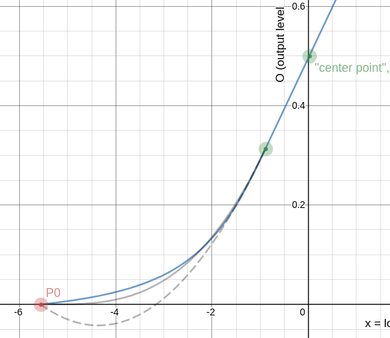
I’ll write a longer post explaining the details in a bit, but here’s a screenshot:
This is the lower roll-off, with the new hyperbolic curve in blue, the original curve (that is: my interpretation of it) in grey, and a second-order curve dashed.
If we extend the lower linear range a bit, it looks like this:
The polynomial overshoots, but the hyperbola does not. The same thing happens if you extend the shadow range to however far down you care to. The hyperbola does not overshoot and simply stretches however far it needs to.
Another nice property: If the gradient of the linear segment is reduced to minimum, the roll-off curve becomes a straight line:
Note how the 4th order polynomial keeps “dancing” around the straight line because it is constrained to arrive with gradient 0.
I’ve even researched an additional parameter onto it to allow to make it more or less “crunchy”, and I put a bunch of adaptive limits/constraints on the input parameters to make it harder (though not quite impossible – yet) to produce impossible or silly curves.
Feedback welcome. As I said, I’ll explain the maths and other details in a bit, in a separate post. Will take a little time to write up everything in human-readable form (that is: for humans who can’t read my handwriting).
The curve looks good but I’m worried by the denominator. How do you make sure b x^2 + x + c \neq 0, \forall x \in \mathbb{R} or at least \forall x \in [0 ; \text{toe}] ?
Yeah but slope = 1 is not really a use case here, so I wouldn’t put too much emphasis on getting a straight line.
I’m starting to wonder if it wouldn’t be possible to keep current 3rd/4th orders and add constraints over the derivatives in the solver (like y''(x) \neq 0 to ensure mononicity and y'(x) > 0 to avoid gradient reversal). So that would yield an optimization more than a solving. Something like that : https://fr.mathworks.com/help/optim/ug/lsqlin.html. The reason is higher order splines should be able to model any “round things”, I don’t like having to divide by a polynomial (mind those zeros and their neighbourhood, that will cause arithmetic problem and float denormals that will slow the vector vode), and so far, the splines are handled uniformly by a vectorized routine of FMA that is very efficient. As much as possible, I would like to stick to polynomials.
As noted in the introduction, BVLS has been used to solve a variety of statistical problems arising in inverse problems. Stark and Parker [15] used BVLS to find a confidence region for the velocity with which seismic waves propagate in the Earth’s core. The upper and lower bounds resulted from a nonlinear transformation that rendered the problem exactly linear, and from thermodynamic constraints on the monotonicity of velocity with radius in the Earth’s outer core.
Imposing conditions on the monotonicity and velocity is spot-on what we try to do here, and since we have a closed form for the desired model, any derivative constraint turns into a simple linear equation going in the matrix, so it’s only a matter of unrolling the algo.
I considered using least squares, but that’s kinda cheating. Almost gave in because the second derivative was resisting for a long time, but I found a closed analytical solution for everything I wanted. I’m about to sit down and write a longer post on it, or several… more later today
So we will have to create an tone curve preset maybe strong and then use opacity as a new global contrast slider??
I’m on board and thrilled that work on DT is striving to push the envelope but really a raw editor with no contrast slider in a current module…it may have been flawed but the combination of the fulcrum and contrast slider in the current CB module were quick and if not correct could often generally produce pleasing results quickly right from the same control that you could be tweaking tones and color……I think it will be missed


 filmic rgb


 (Edit: found this emoticon last week, I just love it… )