Any interest in a "film negative" feature in RT ?

rom9 · June 13, 2021, 9:04pm

Please excuse my math ignorance, what is meant by “integrating” here? It’s not like “the integral of a function” i assume, because we don’t have a function, we just have a bunch of pixels.
Does it mean the median value of each channel? Or the average? Again, sorry for the dumb question

So, if i understand correctly, these types of density measurements are taking different wavelengths into account. And the slopes are affected by these wavelenghts/bandwidths.
So, in our case, it is like saying that the plotted data must be first converted into a specific color profile, and if i’ve chosen the wrong one, the slopes will diverge.
In fact, if i compare my very first mesurements i did, taking the raw data directly without any color profile applied, with the data from the same pictures processed by my camera input profile and then saved to linear sRGB, i get different slopes:

Well… maybe i could try converting to different profiles, until i find one that gives parallel slopes?

Agreed, it would be great if we could achieve a decent result automatically, just by picking the film base color, and then allow for minor adjustments only when needed.

Thanks for all the great info!

I’ll try your conversion method tomorrow. In the meantime, here’s a quick conversion using RawTherapee with FilmNeg. Everything default except some color balance:

jorismak · June 13, 2021, 9:58pm

thanks for your linear scan! Always fun to try on scans from other people.

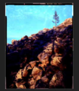
Up front: The relation between blue and red (the rocks and the sky) does seem a bit weird. I can convert it and end up with cyan sky, or I try a different white point and end up with ‘better’ sky on first try, but the rocks can be really red. And very contrasty.

Adding a tiny but of curves to raise the shadows a bit, also lowers saturation (brightening reduces saturation) and it seems ‘better’. Still, a lot of warmth on those rocks .

Also, I do notice something of a limited dynamic range. Not only by looking at the histogram of your linear file, but also when pulling and pushing and working on it, it tends to become noisy if you’re not careful.

I feel your scanner should perform better with the gain raised a bit to maximize DR for your scanner, and I suspect calibration the ‘scan as positive’ with a real it8 slide target may yield interesting results, because something seemed off in your blue/red ratios. Maybe they weren’t all at the same value?

Setting ‘working space’ in Photoshop is always a big no-no to me. It doesn’t really do that much if your files are tagged with a working space, and it seems to confuse people who tend to think it yields better results.

My scans are ‘tagged’ with the profile from calibration. That is converted to rec2020-linear and that’s where I work in. In the end I convert the result to whatever I want for output (mostly sRGB or the profile of my printer).

In your settings yo have ‘blend layers in 1.0 gamma’ enabled. That’s not bad at all, but it’s not the default. Just wanted to point that out :).

whitepoint set on the brightest point in the sky, yielding better sky colors in this case I think.
lce-conversion-example-try1.tif (16.7 MB)

whitepoint set on the brightest point in the picture, which seems to be a specular highlight on one of the rocks.
lce-conversion-example-try2.tif (16.7 MB)

I like to have the ‘reciprocal’ in the method, so I want to do a 1/r 1/g 1/b or something in there.

Working in 16bit Photoshop or 16bit Affinity Photo I switch it around a bit. I find the darkest point in the scan (so what will become our whitepoint in the image). I fill a layer with that color, then place the scan-layer on top of that with the ‘divide’ blend mode. That inverts the picture while having your white point set. After that we still have to set the blackpoint (but you have a bit of filmstrip in your scan for that!). This seems to work better while gamma-corrected. So I apply a dirty levels layer to push the gamma up by +/- 2.2 (a power of 0.45471). Then I add another levels layer and use the black-picker and click on a bit of filmstrip. Or - Affinity Photo ahem, - I add a permanent color-picker on the filmstrip and I adjust black-levels of the R, G and B channels up manually till the filmstrip reads 0,0,0 as values.

‘Basically’ I’m there. In the try1 version I added a little curves to boost the shadows, int he try2 version I did nothing. I used 563/256 = 2.199 gamma now which is the AdobeRGB gamma, but you can adjust it too taste. Or - in my case - the scan images are tagged with a linear ICC profile, so Photoshop and Affinity Photo already display it correctly without having to do a gamma adjustment myself.

I start just like you, with a linear file and while working I add a gaussian-blur (+/- 6px). This removes sample-errors from grain / noise / weird pixels. Using a live-layer or something helps, so you can just ‘turn it off’ in the end.

I add a threshold layer on top, and I set almost as low as it goes. I use this for finding … well, thresholds.

I slowly move the threshold slider up, till black spots start appearing in the image. I ignore parts of your film-leader, we’re only interested in the ‘real image content’. In ‘try2’ I picked this point, the highlight of the rock:

In try1 I used this, in the sky (hoping it would be a white cloud):

I then sample that point (with the threshold of ofcourse). Either sample with the blur layer working, or pick an average 3x3 or 5x5 picker to average it out.

Now, we’re going to create a solid-color fill layer with that selected color, and put it under the scan. We take this color, and divide it by your scan, not the other way around.

Red layer is the new fill solid, with the solid sampled color. Green is your original scanned image, and we set the blend mode of it to ‘divide’.

This already gets us a lot of the way:

I add a levels layer, and give it a gamma correction of +/- 2.2 (depends on the software if you need to enter ‘2.2’ or you need to enter the value of ‘1/2.2’. It should be brighter .

Then I create another levels layer, and adjust the individual channels so that the filmstrip becomes pure black. I need to add a color-sampler to it and watch the values manually:

This yields me the result of ‘try2’:

Turn off the gaussian blur, and you can tweak it further. This is my ‘start’.

In Affinity Photo I can actually do this all in 32bit mode, so I never clip anything. After setting all my thresholds and points, I can always take a levels layer and lower the whitepoint to recover information that might look clipped. This makes setting the whitepoint pure relevant for ‘starting exposure’ and ‘white-color-balance’. So I can try different points to see what color they give, and always lower the exposure again to get everything outside of clipping ranges.

As a trick I learned from @rom9 somewhere in this thread, you can look at the median of ‘the whole resulting image’ (all channels combined), and then add a levels layer, and adjust the gamma of the channels individually till the median of that channel matches the overal median. I think Photoshop has it the histogram view. I know Affinity Photo has it - a bit buggy though.

In try2, that gives me this, a try2b - still the sky is cyan though:

I couldn’t resist and had to try the ‘median color balance’ thing on the ‘try1’ version as well. It turned the blueish sky back to cyan a bit . But it did nice things to the rocks though (not as neutral as previous, but not overly red).

Now, normally I have my own programs to do this in batch. The method I use then is a bit different, but it’s the order of the calculations that’s different, the principle still is the same.

I divide the film color by the scan. That gives me values who start at full clipping white and go up. You can’t do this in Photoshop, you need a good 32bit / HDR workflow for this. Subtracting ‘full white’ from it gives me an image that starts at full black (and the filmstrip should be full black) but goes up into very hard clipping levels. I then scale the whole thing with one big multiplication back into 0.0 - 1.0 range (so nothing clips). Then I look at histogram-binning per channel to set the whitepoint. Since I’m working in HDR, I can be quite aggressive with my percent-thresholding here, because nothing will be truely clipped.

I then do the median-color balance thing (or not, or at 50%…) and can think about saving the file. I can bring everything back into non-clipping ranges and write it as a 16bit TIF file, but it would require some exposure fixes (since I lowered exposure to prevent clipping). Or I save it as a 32bit floating-point tif file, or - even more to my liking - a PIZ-compressed EXR file. Those EXR files open in Darktable, where I can mess with filmic or other tools to map the dynamic range into display-ranges.

The thing here, is that I merge all scans from an entire roll into one big mosaic, of 512x512 squashed images with absolutely no spacing or other pixels in between (and no filmleaders, or sprockets, or whatever). This helps setting the blackpoint/whitepoint And median color balance for the whole roll of film in one analysis. This helps me to disregard outliers in weird scans or pictures. Those auto-tools work really well when you use them on 36 pictures of the same film at the same time (imagemagick’s magick montage is golden here).

In the end I get a bunch of values, which I can enter into an imagemagick commandline to process the individual scans at full resolution.

I’ve been learning g’mic lately and have functions and filters now that do the same thing in g’mic.
I’ve written the tool in c++ as well using libvips that does the whole ‘making montage and analyzing’ thing on a glob pattern of files, and then processes those files with the settings discovered. This automates it pretty well. But it’s harder to experiment with methods so the c++ tool didn’t see much love lately.

nicnilov · June 13, 2021, 10:07pm

“Integrating to grey” in the same sense Hunt uses it in the quote in this earlier post. As far as I understand this just means the compensation of the film channels being apart from each other by the paper response, quoting:

Accordingly, in printing color negatives, it is often arranged that the cyan, magenta, and yellow layers of the print material receive exposures inversely proportional to the red, green, and blue transmittances of the negative, respectively.

Since we don’t have the paper, it should be the algorithm’s task to compensate for the gaps between the channel curves. In order to do that it needs to establish the boundaries of the straight part of the curve and its slope, for each channel. Then, using these values, calculate a correction such that all three curves are aligned along their straight part. This would mean greys along most of the midtone area become neutral, that is, well, grey. That’s what would “integrating to grey” mean in the digital application, I think.

Different coefficients, which yes, seem to end up using different wavelengths, as is shown on this picture (page 4). There is also the formula:

I believe the coefficients above are used as Sr, Sg, and Sb in this formula.

How did you originally measure these values? Was it using a densitometer/colorimeter from film, or from a linear scan on the image data?

Kind of, but the printed density is not color. We still need to calculate the density values similarly to how we calculate a color profile conversion, but the formula is different.

But that’s natural, the application of a color profile modifies the color coordinates in a color space, and that results in different density values, changing the shape of the curve. That is a wrong chart though, this is the right chart:

It does look like something that can be fixed by applying the printing density calculation formula instead of (what could be the default) Status M.

Thanks! This looks much better than what I was able to achieve with FilmNeg. The colors are closer to the digital version too, but the tonal definition is not satisfactory. Is there a way to improve?

nicnilov · June 13, 2021, 10:41pm

Indeed, instead of the channel equalization in Photoshop I did try adjusting the per-channel gain when scanning. This proved to be difficult as it takes many attempts to find the gain values such that the film rebate becomes neutral, otherwise the need for the manual equalization is still there. More to the point, I didn’t notice any improvement in terms of the image quality due to the gain increase. Since it’s a 16bit per channel file, even the narrow histogram has enough variety of values to keep the tonality within reason. So for this scan the gain was the default, same for all channels. With that said, of course it would be preferable to achieve a wider values distribution when scanning.

Regarding the scanner calibration, also a good point, in fact I forgot to mention in the post that a flat field correction along with the scanner profiling should be beneficial for the end result. This example though does not use it.

It’s a valid and quick method but I don’t use it because it can lead to a channel being clipped, depending on the channels relationship. This is easy to miss so I avoid this.

There is no real whitepoint in this image. Everything, including the clouds have chromaticity. This alone makes it useless to rely on any specific image point for correction.

On try1 the rocks look good but I feel there is an overall yellowish tint on the whole image, including the sky. This isn’t right. Also note how the clouds along the rocks line are blown and are likely clipped. Could this be the result of the “divide” blend?

Try2 looks bleached, and like you’re pointed out, the cyan is way too strong.

I do appreciate the attempts though, it helps to find out if there are any missing bits. With that said, the point of this exercise is to demonstrate/improve a correction which is automatable. For this reason no local corrections or anything image-specific should be applied, it’s just wouldn’t be reusable. The point is not to find the best rendition of this particular image, but to find a correction that would work equally well on this, as well as on a completely different image.

nicnilov · June 13, 2021, 10:53pm

The rocks are not neutral in this light, nothing is. More importantly, there are some film defects which maybe several pixels wide, both white and black. This may not be apparent in these smaller files, but should be taken into account when finding the brightest and darkest spots.

That’s maybe where the clipping came from. When the area is blurred, the brightest pixels are dimmed down to the average level in the area. When using a dimmed pixel as a whitepoint, naturally, everything brighter than that gets blown out.

jorismak · June 14, 2021, 7:03am

That’s why I do this normally in 32bit HDR, then you can always after everything is done lower exposure to get clipped values back in range.

And like you said, there is no whitepoint in this image… but you have to set it somewhere. The reason I like to scan/convert a whole roll instead of a single picture. Gives you more possibilities to judge if you set it correctly. With 135 this is easier than sheet… I get 36+ pictures to find a common black/gray/whitepoint .

You used a curves adjustment that you invert. Why not just insert an ‘invert adjustment’, it exists?
Although you can good results (heck, people also had good results by just hitting invert and then hitting auto-levels ) by using a simple 1-i invert, I still think you have to use a 1/i somewhere.
I use the threshold layer to set a point and then divide/invert it. You use the ‘holding-alt while sliding levels’. In the end it does the same thing, it highlights where things start to clip and you stop there. So what clips or not is up to you. And like I said, use 32bit floating-point workflow, nothing can get clipped.
You said you use LAB space to balance your filmstrip to be neutral. Why not just look at the RGB values to see if they match?

And on my personal tastes: An image almost always requires some blacks and some whites. That means that something has to clip a bit, otherwise it looks dull. Those specular highlights, I almost always turn to full white, because otherwise the image always seems to be lacking something. But that’s me, and this is a personal choice.

Looking at the pictures, my ‘try1’ with color-balancing seems very similar to rom9’s ‘FilmNeg + color balancing’. They both seem to ~preserve~ show more details in the sky than your screenshots. If the workflow suites you or not, only you can decide.

Balancing points without having something of a reference is always a pain, and has more to do with your memory of the scene than the picture you took. In digital this is the same if the white balance is completely off and you have nothing to neutralize it against. In film this the same if you have nothing but the blackpoint of your filmstrip.

rom9 · June 14, 2021, 9:18pm

Ok, i tried the LCE method in Gimp, and i think i’ve got the point. In fact, it should be easy to automate, provided that the user will select the “meaningful” area of the negative, excluding any outliers (film holder, sprocket holed, etc.) it’s only a simple histogram analysis.
I’m still not convinced it will work in really unbalanced negatives, with a strong dominant across the entire frame, like a sodium bulb-lit street scene, or a LED-spotlight-infested concert…
Anyway, i can try to implement it.

Related to the paper, i noticed that in the Fuji Crystal Archive paper datasheet you linked above, the characteristic curve plot was missing. Then, googling for the same title, i found this other very similar datasheet, whish has the curve plot, and here it is:

This is completely different from the film response curve! It’s a simple sigmoid, and not mostly a straight line. Notice the size of those toe and shoulder.
So, i implemented the Generalised logistic function in my test program, and actually it feels easier to adjust, compared to other curves i’ve tried before.

No, the film was “scanned” with a digital camera (Sony A7). I have no means of doing any spectral measurements (neither of the illuminant, nor the film or the sensor), so i don’t know where my peaks lie, but sure i can apply those Status A coefficients to my channels… although i think it will be a shot in the dark…

Absolutely, there’s the Tone Curve tool in RT which is very flexible. It works downstream of the filmneg tool, so it can be used normally, as in a digital picture

nicnilov · June 15, 2021, 7:54pm

As it appears, I forgot to mention many important things. LCE will indeed not work well with unbalanced negatives, but there is an objective explanation, and a fix.

By unbalanced negatives we should understand those exposed under a light that differs significantly from the one the film is rated for. For example, consider we shoot a winter scene in the Northern direction on Ektar 100, which is rated for “daylight”. The real temperature for such scene would be way higher. Not unexpectedly, what we get after the LCE conversion is a much stronger cool cast. This is similar to what we’d get with a digital camera set to e.g. 5500K, meaning, the behaviour is predictable, and maybe even useful.

Here is such an example. The correction is exactly the same, except for the dynamic range. Same exact Hue/Saturation adjustment applied here, yet it is obvious it is not enough.
This was shot in February around 13:40, the very end of the afternoon, beginning of the sunset. The sunlight color was probably still pretty “daylight”. The camera is looking North so all the shadows and everything not in direct sunlight should be quite cool (or hot in Kelvin terms).

The fix is either going further with the Hue/Saturation adjustment, and I did that before, or treating the cyan tint as an uncorrected WB, and correct it as such. Here is a cool thing. See what happens if we just change the WB (well, actually also reduce the exposure a bit as in the Camera Raw changing the WB blows the highlights):

Ain’t it nice? So far the theory holds. The correction is still global so should be automatable.

Now that I think of it, maybe the amount of the “residual” cyan cast can be measured and provide an idea of the real scene white balance, a piece of info not otherwise obtainable from the frame.

As an extra, here is what happens when we replace the initial Hue/Saturation with a stronger WB correction, followed by a Hue/Saturation adjustment to reduce the cyan in the highlights:

Note that this may be less representative as this state hits the color space boundaries and the colors change significantly when converted from ProPhoto RGB to sRGB. Also note but disregard the weird shades of the snow in the foreground. This Ektar is expired and that’s how it manifests, the effect is exaggerated by the conversion to sRGB , meaning it’s a different issue.

Another new observation is the Ektar curves. Note how B is not actually parallel to G and R. Maybe that contributes to the extra cyan in the highlights.

Also note the Status M densitometry, as opposed to Printed Density. This does makes sense, as this is what the Status M is for, measuring the film response on its own. The whole system of film/paper should be measured with Printed Density, but not the film individually. Nevertheless, this needs more thinking.

The thing is, film curves actually are sigmoids as well, its just their shoulder is not shown on the charts. I remember reading about it in one of the books, but can’t remember where.

On this chart the channels more or less coincide, meaning the image is balanced. Can it mean a finished print measured for the color reproduction? I’m not sure I understand what does it tell us, could you please explain?

nonophuran · July 3, 2021, 9:04am

Hi everyone,
@rom9, I apologise for getting “lost” again here.

Note: I like medians really, I consider them as a good tool for a WB starting point.

can you remind me how the default median WB (i.e. the one that’s computed when the filmneg module is first switched on) is tied to red and blue ratios?
how hard would it be to have a button to re-compute the default median?

Both questions are related, though in different scenarios.

A. Sometimes, on a roll, I do not have enough suitable neutral tones patches. So I can’t get the red and blue ratios comfortably where they should be. And I’m wondering if their being way off in the first place influences the initial median-based white balance.

B. More frequently, when I find a suitable frame (with nice neutral tones) for initial inversion and replication of settings (copy, paste processing profile, in RawTherapee UI terms) to other frames of the same roll, I find myself unhappy with the median WB value that’s being replicated.

→ do I have a way to re-compute that median, locally, for a given frame (without having to unapply the entire processing profile)?

Thanks.

Ilyaz · July 9, 2021, 3:01pm

Math: Part 0

I’ve read through all the messages on this thread, and it seems that there is a lot of confusion on the math of what happens during the scan. I suspect that this confusion leads to many decisions which lower the quality of the output, make it hard to manually tune the process, and complicate the UI.

To make the long story short, there are the following phenomena (ⓐ ⓑ ⓓ ⓔ match the explanations in the longer versions):

ⓐ There is a cross-talk between the R,G,B channels in the camera. Compensating for this (by a linear mix) may significantly improve “linearity” of the overall process.
ⓑ There is a cross-talk between the 3 pigments in the film. Assuming that ⓐ is done well enough, one can compensate for this by a linear transformation in log- color space. (This has a chance to produce much better color fidelity.)
ⓓ Each pigment has a non-linear response⁰⁾ in shadows (and for some type of film, in the highlights as well). One should compensate for this both for better colors/contrast in shadows, and:
ⓔ … for the calculation of the powers in the power laws (this is currently done via picking light-gray and dark-gray patches).

⁰⁾ Here we assume that the power law is already applied, so the response is ALREADY linear in midtones. So “this non-linearity” is meant to be “on top of the power law”.

“In reality”, there are significant non-linearities involved in parts ⓐ and ⓑ. However, I think I found “a shortcut” which

uses only linear recalculations (combined with conversions to and from log- color-space) to separate colors (actually: separate pigments).
has a good chance to be a MUCH better approximation than what is currently used in RT.
seems to be simple to explain:
(α) Remove the camera colors’ cross-talk by mixing RAW channels with (largish) negative coefficients;
(β) Take logarithms;
(γ) Remove pigments’ cross-talk by mixing new color channels with (largish) negative coefficients;
(δ) Correct curves¹⁾ of non-linearity of the density of each pigment (I mean the curve exposure → density);
(ε) Examine gray points ⇒ multiply by suitable coefficient for each pigment;
(ζ) Return back by taking exponent.
After this the significant part²⁾ of non-linearities is removed, and one can process this as any other RAW image.³⁾

¹⁾ If an unexposed part of the film is accessible, this might be done automatically (given the documentation for the film).
²⁾ If the light source has 3 narrow spectral peaks, this may even remove ALL the non-linearities!
³⁾ Conjecture: with a fourth (infrared???) channel, this would also get the info about the dust.

I already have one part of the longer version written (covering ⓐ and ⓑ). If there is some interest, I would post it soon.

Entropy512 · July 9, 2021, 3:41pm

As far as the camera color channel crosstalk - that’s exactly why raw processors already have matrix-based camera input profiles. It’s also why rom9 states that RT’s white balance should be set such that it white balances the backlight, not the negative.

However you raise an interesting point that perhaps the working colorspace of RT is not the appropriate one for negative inversion. The challenge may be that the appropriate working colorspace for negative inversion is likely film-dependent…

nonophuran · July 9, 2021, 3:44pm

Hi @Ilyaz
Much appreciated. I can only ask for more.
I have a few comments and questions but mostly, I can’t wait for your next post.

damirk · July 9, 2021, 7:42pm

Hello!
I have been following this topic for a long time and agree with @Ilyaz assessment that the problem has not been clearly defined. So, for what it is worth, here are some of my observations (defining the problem the way I see it).

The measured density curves are not parallel, rather they appear as the scaled copies of each other (within the limitation of analog process). I submit that this is by design and applies to all negatives using C-41 process regardless of brand and type of the film. If they were parallel, the distance between them wold be equal to density of the dyes in the orange mask on unexposed areas. In other words, the orange mask would be a constant density overlay which we know is not the case.

After re-scaling of the measured values as per @rom9’s initial premise, the curves do become parallel, separated by the density of the dyes in the orange mask on unexposed areas, and can be removed by simple white balance. Now, if you check figures 5 through 8 in “The Chemistry of Color excerpt.pdf” posted by @nicnilov, you can see this is exactly how the orange mask works.

Please note that simple process for removal of the orange mask is a mayor achievement and @rom9 deserves an extra pat on the back for discovering this.

Next, for white balance, I believe that looking for the neutral patches on the linear portions of the curves is trying to solve two separate problems at the same time.

The first problem is orange mask. The orange mask is removed by white balancing the unexposed area of the film (after re-scaling).

The second problem is spectral mismatch between scene illumination and the film (e.g. daylight - tungsten). After orange mask removal, the negative is balanced to the design illumination for the film (e.g. the daylight film exposed by tungsten light will, after inversion, produce an image with typical orange cast). The reason is that the density curves are misaligned on the scene illumination axis. Therefore, the white balance can align toes and shoulders or straight sections, but not all three (the color temperature setting will not work either as film tone response curves are “baked in”). We need the “curves” tool preferably preset to typical film tone response curve.

Finally, the color profiling is anything but simple as it seems that each roll of film would require a separate color profile for each camera/light setup.

Please do not shoot me if I got any or all of this wrong!

Ilyaz · July 9, 2021, 11:06pm

This is a very frequent confusion on this thread! Note my words above:

After this the significant part²⁾ of non-linearities is removed, and one can process this as any other RAW image.

And this “one can process” involves the matrix profile — but this profile should match the film-layers’ spectral curves, not the camera’s. (The camera’s story ended before the step (β) described above.)

So the pipeline I discussed is completely complementary to the usual RAW pipeline — it doesn’t replace anything in the usual pipeline. These supplementary steps convert one (linear) RAW file (from the camera’s sensels) by another (linear) RAW file (one “captured by the film layers”).

Conclusion: the “whole” pipeline I described has 3 matrix-mixing steps:

To cancel the cross-talk of camera’s sensels (in linear space).
To cancel the cross-talk of film’s pigments (in log-space).
To cancel the cross-talk of film’s layers sensibility (in linear space).

What you wrote matches the third one.

For me, this seems a complete lunacy. Nowhere¹⁾ in the physics of scanning is the backlight relevant — only its “mix” with the film’s base.

¹⁾ … except for the sprocket holes!

Ilyaz · July 9, 2021, 11:30pm

Math: Part I

① The flow of light during the scan of a film goes as this:

Light source creates light intensity depending on wavelength as L(w).
This is filtered through the film base (substrate) with transparency S(w).
This is filtered through the red-capturing pigment with transparency ρ(w)^r; here r is the optical thickness of this pigment.
This is filtered through the green-capturing pigment with transparency γ(w)^g; here g is the optical thickness of this pigment.
This is filtered through the blue-capturing pigment with transparency β(w)^b; here b is the optical thickness of this pigment.
This is caught by a camera sensel with sensitivity C(w) (depending on the type of the sensel).

The resulting effect at wavelength w is L(w)S(w)ρ(w)^rγ(w)^gβ(w)^bC(w). The sensel records the average value of this function of w.

Conclusion Ⓐ: only the product L(w)S(w)C(w) matters, not the individual factors L(w), S(w), or C(w). (Hence it makes absolutely no sense to color-balance light source + camera without taking into account the film’s base.)

Conclusion Ⓑ: if we could manage to make the product L(w)S(w)C(w) “monochromatic” (in other words, to be concentrated at one wavelength w₀ only), then above, instead of “the average value” (which is “very non-linear” in r,g,b) one gets a simple expression L(w₀)S(w₀)ρ(w₀)^rγ(w₀)^gβ(w₀)^bC(w₀). This immediately gives us the linear combination of r, g, b of the form r log ρ(w₀) + g log γ(w₀) + b log β(w₀). If we could also repeat it for two other wavelengths w₁ and w₂, we get 3 linear equations for 3 unknowns, so it would be easy to find the FUNDAMENTAL DATA r, g, b.

Conclusion Ⓑ₁: for best result, one should use monochromatic L(w) (since L is the only parameter one can control). Making 3 photos of the film with 3 different sources of monochromatic light allows a complete reconstruction of r, g and b using a simple matrix algebra.

Conclusion Ⓑ₂: to minimize the “crosstalk between the pigments”, the wavelengths of monochromatic sources should be as widely separated as possible w.r.t. the absorption spectra of 3 pigments. Essentially, this means “w₀, w₁, w₂ widely separated while staying near 3 peaks of the spectra of 3 pigments. (Note: they are not the peaks of sensitivity of the layers of the film!)

Conclusion Ⓑ₃: if one has no control over L, for best linearity one should mix¹⁾ the RGB-channels of the camera so that the mixes have as narrow wavelength-bands of L(w)S(w)C(w) as possible.

¹⁾ In some situations, there are reasons to avoid mixing camera channels with some coefficients negative. Moreover, the situation when the sensitivity C(w) after mixing may take negative values is especially risky. However, the scanned film has quite narrow “output gamut”. Because of this, using negative mixing coefficients is OK as far as all 3 mixed channel in actual film images remain positive. (Having them positive is crucial since the next step involves negative powers!)

Conclusion Ⓑ₄: One should use mixes of RAW RGB-channels R₀,G₀,B₀ like R = R₀ - 0.1 G₀, G = G₀ - 0.1 R₀ - 0.1 B₀, B = B₀ - 0.1G₀. (I expect that 0.1 may be increased even more.)

Conclusion Ⓑ₅: If the light source is mostly concentrated at 3 frequencies not very far from the camera sensels’ peaks of sensitivity, the procedure of Ⓑ₄ can be tuned to match exactly the procedure with 3 monochromatic light sources.

⁜⁜⁜⁜⁜⁜ In what follows, I ignore non-linearities coming from L(w)S(w)C(w) being not narrow-band ⁜⁜⁜⁜⁜⁜⁜

② Note that one can find L(w₀)S(w₀)C(w₀) from scans of the unexposed part of the film. Same for w₁ and w₂. Dividing R, G and B by these “offsets” would “cancel” the effects of backlight+film␣base+camera giving products R’ = ρ(w₀)^rγ(w₀)^gβ(w₀)^b, likewise G’ for w₁ and B’ for w₂.

Conclusion Ⓓ: one can find “the opacity of the red pigment” e^r as a product (R’)ᵏ(G’)ˡ(B’)ᵐ for appropriate k,l,m. Likewise for e^g and e^b with appropriately modified values of k,l,m.

Conclusion Ⓔ: in fact, the effects of cancelling L(w₀)S(w₀)C(w₀) on e^r, e^g, e^b is multiplication by certain constants. So instead of e^r = (R’)ᵏ(G’)ˡ(B’)ᵐ one may use e^r = RᵏGˡBᵐ/c₀, which may be rewritten as (RG^-LB^-M)^-K/c₀. Here the constant c₀ depends only on the type of film (and can be found where r=0: on the unexposed part of film).

Note that considering RG^-LB^-M “cancels the cross-talk between pigments” on frequency w₀, and the exponent -K reflects the power-law dependence of the “sensel output” on e^r.

This finishes the process of reconstructing the density of pigments in the film. Recall the steps:

ⓐ Recalculate RAW channels R₀, G₀, B₀ linearly into “narrow-band” variants R, G, B “cancelling” the RAW channels cross-talk.
ⓑ Calculate the “biased” opacity of each pigment (RG^-LB^-M)^-K, likewise (R^-VGB^-W)^-U and (R^-IG^-JB)^-H (with appropriate K,L,M,U,V,W,H,I,J). This “cancels” the cross-talk between the pigments. (This is linear in log R, log G, log B, r, g, and b.)
ⓒ Calculate the “true opacity” of the pigments (RG^-LB^-M)^-K/c₀ (etc., here c₀ is the value of (RG^-LB^-M)^-K on the unexposed part of the film).

Note that division by c₀ is equivalent to white-balancing in the midtones. Indeed, e^r (etc.) depends linearly on the exposure of film to the (red) light. (This presumes the correct choice of the power K, and holds in midtones, where the law of exposure → opacity=e^r is very close to linear. For many types of film this linearity also works in highlights.)

⁜⁜⁜⁜⁜⁜⁜ How to continue ⁜⁜⁜⁜⁜⁜⁜

③ Explain how to find the cross-talk coefficients L, M, V, W, I, J.
④ Explain how to find exponents K, U, H (essentially, the slopes on the optical density → pigment plots).
⑤ Recalculate e^r, e^g and e^b into the amount of light captured by each of 3 sensitive layers of the film.

However, these are completely different processes, so it is better to postpone them to a different post. Moreover, I see no simple way to do ③ — except for using some “reasonable values”, like 0.1 used in ⓐ :–(.

Ilyaz · July 11, 2021, 12:18am

Have no wish to shoot you (yet)!

Nevertheless, I do not understand this obsession with the color mask(s). For example, above I considered the contribution of film’s pigments as S(w)ρ(w)^rγ(w)^gβ(w)^b, with S describing the transparency of the (intact) color masks, ρ the transparency of 1 unit of the red-capturing pigment, and r the number of units of this pigment (etc).

Of course, what I meant for ρ was “the total contribution” of this pigment — and, in the pedantic mode (one you use! ;–), this contribution consists of two parts:

the pure transparency of the this pigment ρ_p(w);
the cancellation of opacity ρ_m(w) of the mask.

Assume that 1 unit of this pigment eats ⓡ units of the mask. Then the total contribution of this unit into film’s transparency is ρ_p(w)ρ_m^-ⓡ(w). Hence the contribution of r units is (ρ_p(w)ρ_m^-ⓡ(w))^r.

Conclusion: proceeding in the pedantic mode is equivalent to using ρ(w)=ρ_p(w)ρ_m^-ⓡ(w) in the “naive” mode of my notes above/below.

damirk · July 11, 2021, 2:46pm

@Iliaz, I have a problem with your explanation: the mask pigments are not in the image making layer of the same color. In other words, the yellow mask pigments are in the magenta layer and are destroyed by magenta density (green light), while the yellow mask pigments are in the cyan layer and are destroyed by the cyan density (red light). In other words, the light creating the image layer and light destroying the mask layer are from the different part of the spectrum and the ratio of image creation and the mask destruction varies from point to point depending on the color composition of the light falling onto that point of the film. So, while mask and image density pigments are measured together they are independent from each other.

One can look at the orange mask as an analog implementation of the camera profile: film camera has film as a sensor, so, as the sensor changes with every roll, it makes a lot of sense to bake the profile into the film. Thus removal of the orange mask is a necessary step irrespective of whatever else we do.

Rick · July 11, 2021, 6:32pm

I thought about starting a new thread, but then saw this one. I’m just now getting into DSLR scanning (in my case, a mirrorless Fuji X-T4). This is my first attempt. While I mostly like the results, it was some trial and error to get here. And some color tweaking in RT (courtesy of LAB adjustments). Thankfully the grain tank in the background offered up something resembling neutral gray for the white balance. Interestingly, these same settings didn’t transfer well to other frames shot on this same roll and scanned with the same settings.

More info: My blog post.

jorismak · July 18, 2021, 8:43am

I do think that if other shots on the same roll, taken at roughly the same point in time and same lightning conditions, scanned (shot with Dslr in your case) the same and processed the same, they should develop pretty much the same.

I choose one process setting (as a starting point at least) for an entire roll all the time.

You’ll see the exposure differences between the shots, which can explain why some have a slightly different color balance. But mostly if I have one, I have the entire roll.

Differences occur when a part of the roll is shot inside VS other shots outside. Or if I let the roll sit in the camera, and a few months have passed between shooting the first half and the 2nd half for example.

I see a lot of people with film scanners or Dslr-scanning who have some sort of auto exposure enabled during scanning, and with a Dslr do not use the exact same Dslr settings for the entire roll… This will of course give differences frame to frame.

Personally I take the scans of a roll, crop them, and then make a collage of all the scans without any room between the shots. So I force-resize all the scans to 512x512 as example (yes, messing with the aspect ratio) and glue them all together.

I then process that collage as a single image to determine a balance that seems to fit the entire roll. I then take the original scans and process them with exactly the same parameters to get my ‘starting point images’.

Rick · July 18, 2021, 2:37pm

That mostly makes sense, and I think I can reproduce a similar process. I’ve been manually setting my WB when scanning, but what I’ve also relied on auto exposure. That will of course change from frame to frame with each given density. I’ll make an adjustment and go from there. Thanks for the feedback.