Here, try reading this thread: How to export animation via gmic cli [SOLVED] - #8 by grosgood
The closest to real time animation is to use window command. You did it before, I think.
Here, try reading this thread: How to export animation via gmic cli [SOLVED] - #8 by grosgood
The closest to real time animation is to use window command. You did it before, I think.
Ditto.
See “Simple particle system” in @David_Tschumperle 's Post 171, Big Bad Thread of Silly Questions. Look at the code after the #Render animation comment.
Well, I sometimes use window to check my loops and it sometimes does animation.
But anyway, wasn’t that what @Reptorian was asking here? ![]()
I think I have it.
For now, it’ll do for me, but it still needs way, way, way more work
Here it is:
$ 100,100,100,4,v=norm(x-49.5,y-49.5,z-49.5)/50;v<1?lerp([0,1,1,255],[360,1,1,255],v); hsv2rgb rep_preview_3d_animation
#@cli rep_preview_3d_animation: '_fps>0'
#@cli : Previews 3D images as animations via windows.
rep_preview_3d_animation:
skip ${1=30}
check "$!<10&&$1>0&&isint($1)"

delay_time={int(1000/$1)}

num_of_windows,screen_w,screen_h=$!,{*,u},{*,v}
+store temp

scaled_screen_w,scaled_screen_h={int([$screen_w,$screen_h]*.9)}

foreach {
 if w>$scaled_screen_w||h>$scaled_screen_h
  r2din $scaled_screen_w,$scaled_screen_h,3
 fi
 +crop 0,0,0,0,100%,100%,0,100%
 drgba.
 w$>. -1,-1,0,0,50%,50%  rm.
}

$!,1,1,2,[1,d#x] => frames_data

do
 repeat $num_of_windows {
  current_frame,number_of_frames:=I[#$frames_data,$>]
  +crop[$>] 0,0,$current_frame,0,100%,100%,$current_frame,100%
  drgba.
  w$>. -1,-1,0,0 rm.
  set. {($current_frame+1)%$number_of_frames},$>
 }
 wait $delay_time
while {*}

rm $temp
Didn’t really know that’s a thing. I keep getting errors with it though, so I don’t know if that command is suitable for my needs.
C:\Windows\System32>gmic 100,100,100,4,v=norm(x-49.5,y-49.5,z-49.5)/50;v"<"1?lerp([0,1,1,255],[360,1,1,255],v); hsv2rgb animate3d 1,1,1,1,1,1
[gmic]./ Start G'MIC interpreter (v.3.3.4).
[gmic]./ Input image at position 0, with values 'v=norm(x-49.5,y-49.5,z-49.5)/50;v<1?lerp([0,1,1,255],[360,1,1,255],v);' (1 image 100x100x100x4).
[gmic]./ Convert color representation of image [0] from HSV to RGB.
[gmic]./ Generate 3D animation frames from 3D object [0], with 1 frames, angle steps (1,1,1), zoom factor 1 and 1% fake shadow.
[gmic] *** Error in ./animate3d/*repeat/*local/ *** Command 'check': Expression '0' is false.
animate3d can be used for 3D-vector objects, not 3D volumetric images.
Also, it does generate frames of an animation (e.g. to save a video), this is not what you are looking for.
In your case, it seems you are talking about visualizing a 3D volumetric image in 3D.
There is multiple ways to do that, and all depend on the content of your volumetric image.
For your example, command pointcloud3d may be useful.
But remember, as your volumetric image is dense, you’ll see probably mostly the outer surface of your image, not the interior, unless you make your 3D object semi-opaque (opacity3d).
How can I get this to work?
$ m foo:continue repeat 1000 { echo 1 foo echo 2 }
I know why it won’t though.
And yes, I know of the single variable trick. Hmmm…
Right now, I’m suspecting that +pal code can be shortened with base642uint8, but without the feature idea I had in mind, it’s not possible. Or maybe I will create a new code copying from base642uint8 to find a workaround.
This won’t work because when you call foo , you’re entering a new command, and in this new command the continue has no sense (you’re not inside a loop in this new command).
That’s actually the difference between a command and a macro (macro functions is the things you can define in math expressions, but you cannot define such macros for a regular G’MIC pipeline).
And I’d say, fortunately so: If such a continue would have an effect on the “parent” loop, I imagine the nightmare for debugging things.
Yeah, I know that. Now, I tried testing a new approach to see if it would save time (only slightly), but all it saved number of characters from 128000 to 41000. Never mind.
How does one check if a command exist? I think I have a way to make cli_end, which is the opposite of cli_start.
If cli_end exists, then _display will execute it at the very start. This will very easily allow me to separate my user.gmic files entirely.
I wonder if parse_cli can find it?
Probably something as:
if ['$$cli_end']!=0 ... fi
(but works only for custom commands).
Thanks, that works. I inserted this under _display code at the very beginning:
if ['$$cli_end']!=0 cli_end fi
And added this to user.gmic
cli_end: blur 100
And running $ sp cat will show me a blurred image. This definitely will allow me to just simply import .gmic script, and execute __main__ without having to type __main__ on the CLI if it exists on the imported .gmic script.
I’m not getting the same result here:
Python:
def compute_fft_simple(image):

    # Load the image and convert to grayscale
    img = image.convert('L')

    # Convert image to numpy array
    img_array = np.array(img)

    # Compute the 2-dimensional FFT
    fft_result = np.fft.fft2(img_array)
    magnitude_spectrum = np.abs(fft_result)
G’MIC
to_gray
+fft
a[-2,-1] c
100%,100%,100%,1,cabs(I#-1)
rm.. log.
And yet, I think these output are the same with smaller images:
>>> import numpy
>>> a=numpy.mgrid[:5,:5][0]
>>> a
array([[0, 0, 0, 0, 0],
       [1, 1, 1, 1, 1],
       [2, 2, 2, 2, 2],
       [3, 3, 3, 3, 3],
       [4, 4, 4, 4, 4]])
>>> fft_result=numpy.fft.fft2(a)
>>> fft_result
array([[ 50.  +0.j        ,   0.  +0.j        ,   0.  +0.j        ,
          0.  +0.j        ,   0.  +0.j        ],
       [-12.5+17.20477401j,   0.  +0.j        ,   0.  +0.j        ,
          0.  +0.j        ,   0.  +0.j        ],
       [-12.5 +4.0614962j ,   0.  +0.j        ,   0.  +0.j        ,
          0.  +0.j        ,   0.  +0.j        ],
       [-12.5 -4.0614962j ,   0.  +0.j        ,   0.  +0.j        ,
          0.  +0.j        ,   0.  +0.j        ],
       [-12.5-17.20477401j,   0.  +0.j        ,   0.  +0.j        ,
          0.  +0.j        ,   0.  +0.j        ]])
>>> magnitude_spectrum=numpy.abs(fft_result)
>>> magnitude_spectrum
array([[50.        ,  0.        ,  0.        ,  0.        ,  0.        ],
       [21.26627021,  0.        ,  0.        ,  0.        ,  0.        ],
       [13.1432778 ,  0.        ,  0.        ,  0.        ,  0.        ],
       [13.1432778 ,  0.        ,  0.        ,  0.        ,  0.        ],
       [21.26627021,  0.        ,  0.        ,  0.        ,  0.        ]])
$ 5,5,1,1,y +fft a[-2,-1] c 100%,100%,100%,1,cabs(I#-1) rm..
What’s going on?
Agree:
G’MIC:
$ gmic run '5,5,1,1,y +fft a[-2,-1] c 100%,100%,100%,1,cabs(I#-1) a={-1,@0--1:5} e "Column Zero: "$a'
[gmic]./ Start G'MIC interpreter (v.3.3.6).
[gmic]./run/__run/ Input image at position 0, with values 'y' (1 image 5x5x1x1).
[gmic]./run/__run/ Compute fourier transform of image [0] with complex pair ([0],0).
[gmic]./run/__run/ Append images [1,2] along the 'c'-axis, with alignment 0.
[gmic]./run/__run/ Input image at position 2, with values 'cabs(I#-1)' (1 image 5x5x1x1).
[gmic]./run/__run/ Set local variable 'a=50,21.266271591186523,13.143278121948242,13.143278121948242,21.266271591(...).
Column Zero: 50,21.266271591186523,13.143278121948242,13.143278121948242,21.266271591186523
Python/numpy:
gosgood@bertha ~ $ ipython
Python 3.11.8 (main, Apr 14 2024, 01:28:20) [GCC 13.2.1 20240113]
Type 'copyright', 'credits' or 'license' for more information
IPython 8.22.2 -- An enhanced Interactive Python. Type '?' for help.

In [1]: from PIL import Image
In [2]: import numpy as np
In [3]: agrid=np.mgrid[:5,:5][0]
In [4]: fft_result=np.fft.fft2(agrid)
In [5]: magnitude_spectrum=np.abs(fft_result)
In [6]: magnitude_spectrum[:,0]
Out[6]: array([50.        , 21.26627021, 13.1432778 , 13.1432778 , 21.26627021])
However, in general, GMIC to_gray ≠ PIL Image.convert("L"), because their RGB ⇒ GRAY weights seem to differ. They don’t play the game in quite the same way:
to_gray is a wrapper around luminance; it performs image sanity checking before calling luminance for conversion.R=[255,0,0], G=[0,255,0] and B=[0,0,255] I estimate weights R=\frac{76}{255} ≈ 0.29803 , G=\frac{150}{255} ≈ 0.58824 , B=\frac{29}{255} ≈ 0.11373 , so, generally, G’MIC and PIL do not furnish FFT exactly the same data sets. Pretty close. Not ditto. Illustration:test.png:

PIL:
gosgood@bertha ~/git_repositories/gmic/src $ ipython
Python 3.11.8 (main, Apr 14 2024, 01:28:20) [GCC 13.2.1 20240113]
Type 'copyright', 'credits' or 'license' for more information
IPython 8.22.2 -- An enhanced Interactive Python. Type '?' for help.

In [1]: import numpy as np
In [2]: from PIL import Image
In [3]: testimg=Image.open(r"/dev/shm/test.png")
In [4]: bwimg=image.convert("L")
In [5]: bwimg.im.getextrema()
Out[15]: (0, 216)
GMIC:
gosgood@bertha ~/git_repositories/gmic/src $ gmic /dev/shm/test.png to_gray. e "Range: "{im},{iM}
"
[gmic]./ Start G'MIC interpreter (v.3.3.6).
[gmic]./ Input file '/dev/shm/test.png' at position 0 (1 image 128x128x1x3).
[gmic]./ Force image [0] to be in GRAY mode.
Range: 0,241.17601013183594
All that said about RGB ⇒ GRAY, I don’t see alarming differences in behavior from the two environments:
tropic.png (pixelated native under a palm tree):
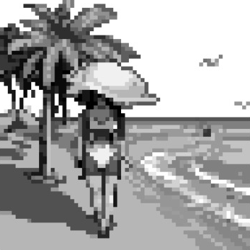
Python, PIL, numpy:
Probably should note the imports on the Python, PIL, numpy side (which were accidentally cropped out):
In [1]: import numpy as np
In [2]: from PIL import Image
In [3]: import matplotlib.pyplot as plt
…
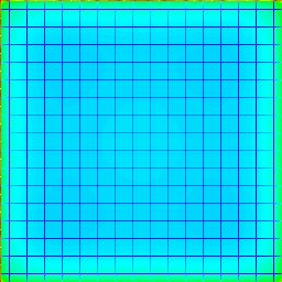
On the G’MIC side:
gosgood@bertha ~/git_repositories/gmic/src $ gmic run '-i /dev/shm/tropic.png to_gray. +fft. a[-2,-1] c 100%,100%,100%,1,cabs(I#-1) keep. log. n. 0,255'
[gmic]./ Start G'MIC interpreter (v.3.3.6).
[gmic]./run/__run/ Input file '/dev/shm/tropic.png' at position 0 (1 image 353x353x1x1).
[gmic]./run/__run/ Force image [0] to be in GRAY mode.
[gmic]./run/__run/ Compute fourier transform of image [0] with complex pair ([0],0).
[gmic]./run/__run/ Append images [1,2] along the 'c'-axis, with alignment 0.
[gmic]./run/__run/ Input image at position 2, with values 'cabs(I#-1)' (1 image 353x353x1x1).
[gmic]./run/__run/ Keep image [2] (1 image left).
[gmic]./run/__run/ Compute pointwise base-e logarithm of image [0].
[gmic]./run/__run/ Normalize image [0] in range [0,255], with constant-case ratio 0.
[gmic]./ Display image [0] = '[cabs(I#-1)]'.
…

So, my take: numerical differences in the details in that the two environments treat gray scale conversions a little differently. Not so big a difference as to change behavior in the main.
Am I missing what you were trying to point out?
Yeah, why is there borders on the Python FFT example?
The full code is this:
def compute_fft_simple(image):

    # Load the image and convert to grayscale
    img = image.convert('L')

    # Convert image to numpy array
    img_array = np.array(img)

    # Compute the 2-dimensional FFT
    fft_result = np.fft.fft2(img_array)
    magnitude_spectrum = np.abs(fft_result)

    # Find minimum value
    is_below_min = magnitude_spectrum <= np.min(magnitude_spectrum)

    # Calculate horizontal tiles
    diffs = np.diff(is_below_min.astype(int), axis=1)
    section_starts = (diffs == 1).sum(axis=1)
    sections_h = (np.median(section_starts) + 1)

    # Calculate vertical tiles
    diffs = np.diff(is_below_min.astype(int), axis=0)
    section_starts = (diffs == 1).sum(axis=0)
    sections_v = (np.median(section_starts) + 1)

    # Resize the image accordingly
    return image.resize((round(img.width / sections_h), round(img.height / sections_v)))
I suspect it has to do with <=, but I will check with the using np.convert(“L”) weighs on RGB to grayscale.
Oh, I forgot to comment on this, but it looks like Garry responded.
The grid, or something else?
Grid.
That’s because tropic.png is made up of squares, all about 6x6 pixels, so that every transition of gray occurs at multiples of 6 along both x and y; this reinforces strong 6k cycle signals in the temporal data for k ∊ {1,2,3…}. This is the sort of periodic behavior that a Fourier transform to the spectral realm will pick up. It shows up prominently in the transition from temporal to spectral representation as distinct “spectral lines” at multiples-of-six frequency coefficients in both spectral x and y; these criss-cross to form the grid. Any checkerboard-like pattern in the temporal realm will produce similar grid-like patterns in the spectral realm. Here is an extreme example:
gmic run '256,256,1,1,xor(x,y) % 32 < 16 n. 0,255 blur 1 +fft. a[-2,-1] c 100%,100%,100%,1,cabs(I#-1) log. n. 0,255 map. hsv'
The slight blurring in the temporal spreads the spectral coefficients a bit, making the grid lines a little wider, as the frequency coefficients get spread around too.
Now for a fun side trip. Mucking around with modulo arithmetic and doing temporal => spectral conversions is a fascinating source of patterns:
gmic run '2048,2048,1,1,xor(x,y) % 30 < 17 n. 0,255 blur 1 o. /dev/shm/temp.jpg,80 +fft. a[-2,-1] c 100%,100%,100%,1,cabs(I#-1) log. n. 0,255 map. aurora o. /dev/shm/spec.jpg,80'
temp.jpg
spec.jpg
Maybe you can have some fun with that.


