Which is - what? - 3.47e+06 items long? ![]()
1 Like
Approximately  . But as it’s an unordered list, there is still hope!
2 Likes
Good observation. It occurred to me for a sec (the mention of SVD gave me the hint) but I completely forgot about it to mention it. It definitely changes things. When brute or naive force doesn’t work, we have to step back and be more intentional or creative.
It is fun following this thread. Keep it up everyone!
Very cool!
You could post your rwcimg module in a Github Gist or new Github project; with very few explanations if you lack time available… For, such a piece of code may be useful for random people in the future, hanging on the internet. Especially, there are few Python x G’MIC pieces of code out there (appart from people calling the G’MIC executable with a Python subprocess call, which is now not so useful with gmic-py).
1 Like
Alright. I’ve had my bus ride. Only screwed up my diagram of the Hamiltonian two or three times, so what do I know? But, at any rate, here I go, racing in where angels fear to tread…
hyp_img={sqrt(sqr(w)+sqr(h))}
n={int(sqrt(($hyp_img^2)/2))}
Bit roundabout. Consider that seed images are square, that w=h. Thus, hyp_img=(2w^2)^0.5. To get to n, you first square hyp_img: now you have 2w^2. You divide that by two: now you have w^2. You take the square root: now you have w, which you set to n. You’ve taken the scenic route. Most cads would have set n=w (or n=h, seed images being square) right off the dime - and then would have been done with it. They have no sense of romance, of poetry. Pox on them.
One way or another the first key metric, N=n=w (or h) has been set to the length of the side of the seed image. This N is a key measure of your Hamiltonian matrix image, for its sides and diagonal are N*N.
npts={sqr($n)}
npts_n={$npts-$n}
npts_1={$npts-1}
You’ve got the pixel count, based on N*N, which, after seed map unroll, is also the length of the main Hamiltonian diagonal: npts=N*N. You’ve got the length of the immediate off-diagonal: npts_1=N*N-1. And you’ve got the length of the diagonal offset from the main by N: npts_n=N*N-N, or N*(N-1), to be undistributive about it.
So far, so good.
200,1,1,1,":begin(const ww=w-1);lerp(0,1,x/ww)"
You are starting to go into the weeds: making use of a derelict intensity ramp based - at some obscure point in @weightt_an’s script development - on a fixed N=200, which is (most likely) not your N.
About the derelict ramp: Your code quite nicely reproduces the numpy function np.linspace(), but - Alas!! - on the Python side, in @weightt_an’s script, the use of that function and the ramp it creates effectively goes unused: debris left over from an aborted experimental direction. Note that @weightt_an is self-studying Python and fooling around with quantum mechanics. Some people just have all of the fun. But in the course of having all of the fun, @weightt_an is trying this out, and trying that out, and leaving the debris of old experiments lying around. One piece of debris makes for yet another bit of roundaboutism. That is, making an entire 200 step linear intensity ramp just to take one step, which works out to 1/(N-1) for an N-step ramp - squares it, and sets it equal to increment. Most cads would have just written:
increment=1/(N-1)^2
incrementValue=-(N-1)^2
zeroV=4*(N-1)^2
and be done with the ramp entirely. But they have no poetry in their souls. In contrast, @weightt_an builds an entire derelict ramp, you drive up onto it, and we all have a good jolly laugh as you go off the top end and into the Hudson - or whatever dank, urban river serves in your locale. Because in taking a one delta step sample from a ramp based on N=200:
increment='{sqr(i(#-1,1))}'
incrementValue='{-1/$increment}'
zeroV='{4/$increment}'
diag0='{vector(#$npts,$zeroV)}'
are now all based on a Hamiltonian matrix for N=200, which is (probably) not the N of your Hamilton matrix, based as it is on the length of the seed image side and from which npts, npts_n and npts_1 derive.
Mismatch. And that, as we Americans say, is the ball game.
2 Likes
Good suggestion. I don’t have nearly the to-do list as @David_Tschumperle, but I sorted mine. By priority. I’ll learn one of these days…
2 Likes
I wanted users to have the option to use non-square seed image. Hence, why you’re seeing hyp_img, and the initial n being based off solving b for a=sqrt(2b^2). Non-square images is not quite the correct way of using this script, but eh I don’t really care about whether users will use a square image or not, and I do know how to create the option of forcing a non-square image to be a square seed.
I did that, it still doesn’t seem to work.
In addition, that can be simplified to:
NN=(N-1)^2
increment=1/NN
incrementValue=-NN
zeroV=4*NN
Here’s the new code which is a lot easier to read.
rep_hamiltonian:

repeat $! l[$>]
 if s>1 to_gray. fi
 ge. {avg(im,iM)}

 hyp_img={sqrt(sqr(w)+sqr(h))}
 n={int(sqrt(($hyp_img^2)/2))}
 nn={($n-1)^2}
 npts={sqr($n)}
 npts_n={$npts-$n}
 npts_1={$npts-1}

 increment={1/$nn}
 incrementValue={-$nn}
 zeroV={4*$nn}

 $npts,$npts

 $npts,5,1,1,"begin(
   const inc_v="$incrementValue";
   const zv="$zeroV";
   cv=[crop(#-2)];
   initial_pos_x=[0,0,0,1,"$n"];
   initial_pos_y=["$n",1,0,0,0];
   v(a)=inc_v*cv[a];
  );
  y==2?(
   i(#-1,x,x)=zv;
  ):(
   pos_x=x+initial_pos_x[y];
   pos_y=x+initial_pos_y[y];
   i(#-1,pos_x,pos_y)=v(x);
  );"
 k..
 eigen.
 k.
endl done
Also, this doesn’t work either:
 increment={(1/($n-1))^2}
 incrementValue={-1/$increment}
 zeroV={4/$increment}
EDIT: unroll instead of crop does not work either. I’m stumped.
1 Like
I’ve been able to implement a first version of the Arnoldi method for approximation of the largest eigenvalues of a large matrix. Looks good (and fast  ).
).
I’ll try to make a version of it working as eigen, and another version working as eig() in the math parser.
Stay tuned!
2 Likes
So… I’ve added a command meigen in the stdlib, that approximates the m largest eigenvalues of a square matrix (passed as a selection of the command). It’s really faster than computing all the eigenvalues, but it computes only an approximation of the eigenvalues (the bigger ‘m’, the better approximation). Also, it does not return the associated eigenvectors.
Some examples of timing on my machine:
- Approximation of the 64 largest eigenvalues for a 1024x1024 matrix takes
0.181 seconds(whileeigentakes36.09 seconds). - Approximation of the 32 largest eigenvalues for a 9000x9000 matrix takes
9.288 seconds.
I’ve also added a new equivalent math function meig(A,m,n) that returns a vector(#m) of the approximated eigenvalues from the square matrix A (with size n x n). Include math_lib in your expression to be able to use it.
At this point, I want to say that:
- I’ve not tested it thoroughly (just on random matrices). Not sure how it behaves with ill-conditionned matrices.
- I hope this will be useful for you, to solve the OP initial problem. I haven’t followed all the discussion, so I can’t really tell. Let me know if you succeed in using it.
- If you’re interested by how I did it : https://github.com/dtschump/gmic/commit/178a52a6bd1fde6c0eda58d6939fc3e97a83498f
And of course, as always, a $ gmic update will be necessary to get this new command.
4 Likes
Ah me. Time to rename G’MIC as ‘David’s Delightful Distraction Machine.’ Methinks he worked past midnight. I’m five hours behind CET…
Five hours behind him, I’ve been fooling around with a diagonalizer.
- It starts with images of arbitrary dimension and spectra.
- Take the lumenance, threshold it to make the seedmap image, then unroll it.
- It is my wont to interpret this as the smallest, most offset +/- diagonal.
- Calculating N is a two-stepper.
a. Find the ‘ideal N’ by the quadratic formula.
b. It has a fractional part, almost always. I prefer to round this ‘ideal N’ up to the next highest even number, and declare this to be N. I find that even N makes padding and positioning these diagonals somewhat more tractable later on. - Having rounded up N, it is necessary to resize the length of the smallest diagonal so that it matches. N*(N-1) tells me what the new length is. It is resized without interpolation and periodic boundary policy; might be more appropriate to change that to black fill policy instead, though no harm seems to come of it.
- The lesser diagonal is essentially a copy of the smallest diagonal, resized to N^2-1, no interpolation and periodic boundary policy as before.
- The main diagonal, N^2 is created and filled with 4*(N-1)^2
- The the offset diagonals are scaled by -(N-1)^2
- Applied
-diagonalto convert these three vectors to diagonal matrices. Though disassembled, and of different sizes, The data for the upper diagonal of the Hamiltonian is in hand. It is necessary to duplicate, pad and shift the two offset diagonals so that, later on, they can be added to the main diagonal. - There follows finicky bits of matrix copying, expanding by xy and cropping to position the off-diagonal matrices to be in their appropriate places, adding the pipeline together, consolidating to a single image, the Hamiltonian, which I wrote out as a float
.cimag
@David_Tschumperle’s brand new toys (!!!) notwithstanding, I harnessed the Python side to find select eigenvectors, to minimize testing to just the diagonalizer. I asked for five solution vectors, exporting the solution eigen_vectors to output .cimg files for post-processing. Runs for N=130 was about thirty seconds.
Using this seed image:

I obtained these select images (filtered by post-processing, given below)
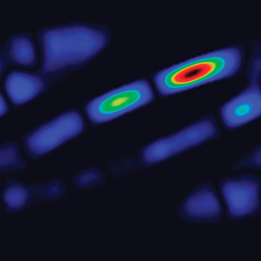
vector_0, N=130, scaled up to 512 and colorized via -map rainbow.

vector_1, the next door neighbor..
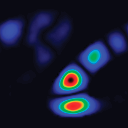
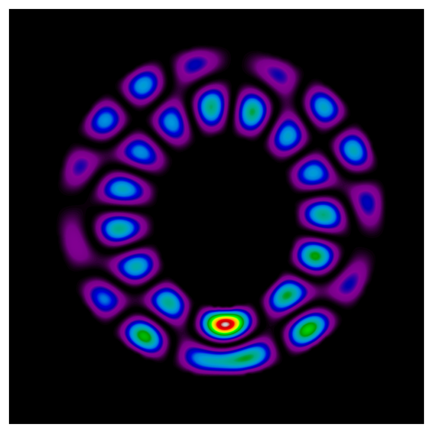
vector from a smaller seed image of the torus, N=75, scaled up and colorized as the others.
This is the diagonalizer:
gmic                                            \
   -input quantum_torus.png                     \
   -luminance.                                  \
   -threshold. 50%                              \
   -unroll. x                                   \
   hy='{(1+(sqrt(1+4*w)))/2}'                   \
   n='{round($hy/2,1,1)*2}'                     \
   nn='{($n-1)^2}'                              \
   iv='{-$nn}'                                  \
   zv='{4*$nn}'                                 \
   -resize. '{$n*($n-1)}',1,1,1,0,2             \
   -mul. '{$iv}'                                \
   +resize. '{$n^2-1}',1,1,1,0,2                \
   -reverse                                     \
   -input '{$n^2}',1,1,1,'{$zv}'                \
   -name. diag0                                 \
   -move.  0                                    \
   -diagonal                                    \
   -expand_xy. '{$n}',0                         \
   +crop.   '{$n}',0,'{w-1}','{h-$n-1}',0       \
   -name. diagmN                                \
   -move. 0                                     \
   -crop. 0,'{$n}','{$n^2-1}','{h-1}',0         \
   -name. diagpN                                \
   -expand_xy.. 1,0                             \
   +crop..   1,0,'{w}','{h-1}',0                \
   -name. diagm1                                \
   -move. 1                                     \
   -crop.. 0,1,'{w-1}','{h}',0                  \
   -name.. diagp1                               \
   -add                                         \
   -output. hamilton_test_'{$n}'.cimg,float     \
This is the post processor:
gmic                                            \
   -input hamilton_test_130_out_0.cimg          \
   '{sqrt(h)}','{sqrt(h)}',1,1                  \
   -fill. [-2]                                  \
   -sqr.                                        \
   -normalize. 0,1                              \
   -pow. 0.75                                   \
   -r2dx. 512,5                                 \
   -normalize. 0,255                            \
   -map. rainbow                                \
   -display                                     \
   -output. hamvecm_0.png
I find the shapes eerie, compelling and interesting. Even with a known seed map, it is not quite certain what the solution vectors will look like.
Next step is to disconnect the Python bit and run with @David_Tschumperle’s new toys. Then we have an end-to-end G’MIC pipeline. Doubt that the diagonalizer is optimal; certainly could use a fresh pair of eyes. Memory usage balloons at one point to 16GB, for N>=150, so it won’t run on Granny’s Tandy TRS-80, probably.
That’s it for now. Everybody have fun.
3 Likes
I’m pretty sure your algorithm is broken somewhere. Well, or I inattentively read your post and you introduced some new settings
My pictures with this seed


2 Likes
Think you are right. Looks like horizontal scaling may be taking place. Thanks for raising the flag. Not sure when I can act on it though.
Probably not going to play in this sandbox for the first half of this week - Real Life chores and obligations press.
- As @weightt_an points out, there are (probable) distortions in how I’m rendering a eigen_vector compared to how his script renders it out. My suspicions run toward the initial calculation and rounding of N that I do. That, and the padding out of the offset diagonals when it comes to boundary policy. Currently I use periodic. That actually adds coefficients to the matrix not in the original unrolled image. Plausible, then, that in effect I make a slightly different seed well than what @weightt_an does. Solution to that is to switch to Dirichlet Boundary policy - i.e. consider off-image pixels as black. That adds no coefficients not already present in the original unrolled image.
- My diagonalizer can put up to five huge images on the image stack at one time. These are related to consumption of up to a 16 GB bulge. I like @Reptorian’s diagonalizer because it writes to one large image from smaller sources. Still think it is worth some time and energy to track down what’s going on with that approach because it is the more memory friendly one.
- Even with a defective diagonalizer, it is not that far away to hook together a G’MIC only pipeline. If somebody else doesn’t beat me to it, that would be my next destination on my a periodic bus trips to Schrodinger’s Well. Have fun!
@grosgood I"m wondering if you could dump the vectors utilized by @weightt_an python script and reveal the value of vectors. I would like a .zip of cimgs to see where I went wrong. If I could compare the values, I might be able to fix my script.
- I’ll use the seed image in post 92. The torus.
- I’ll use N=30 so that the Hamiltonian will only be 900,900,1,1
- I’ll generate the Hamiltonian from his script, which utilizes scipy.sparse.diags()
- I’ll save that out as
ham_N90.cimgand zip it up, posting the zip file here.
Not right now, though. Doing pay work. probably 6 hours from now, my evening.
Well, about 4 hours. They canned a meeting on me. I’m imperfectly disappointed.
Here goes:
well image = quantum_torus_small.png 30,30,1,1
N = 30
No_points N*N = 900
increment 1/(N-1)^2 = 0.0011890606420927466
incrementValue -(N-1)^2 = -841.0
zeroV 4*(N-1)^2 = 3364.0
The diagonals offset from main diagonals have two values, 0 or -841. The main diagonal has a value of 3364. These values are consistent with those computed above.
The first non-zero pixels for the five diagonals are:
diagmN 73,103             (diagonal begins at 0,30. Initial interval of zero-valued pix: 73)
diagm1 73,74              (diagonal begins at 0,1.  Initial interval of zero-valued pix: 73)
diag0  0, 0
diagp1 74,73              (diagonal begins at 1,0.  Initial interval of zero-valued pix: 73)
diagpN 103,73             (diagonal begins at 30,0. Initial interval of zero-valued pix: 73)
These are consistent with quantum_torus_small.png. It’s first two rows are black (60 pixels) the third row is black from zero to twelve (13) 30 + 30 + 13 = 73
The well image, the Hamiltonian generated with @weight_an’s script, and 30 rendered eigenvectors, also computed from his script, scaled from 30->128, normalized and mapped with rainbow.
hamneigs.zip sha256 hash 0d95f76775232a6aedb8a3a6463eadc6cb9fbb060987c39f164ab6ca88e5ad96
Have fun.
hamneigs.zip (434.5 KB)
…I prefer to round this ‘ideal N’ up to the next highest even number, and declare this to be N…
…It is resized without interpolation and periodic boundary policy…
Better to round to the nearest than rounding up. This was adding two: N=s+2 instead of N=s for square images of dimension s. Changed boundary policy to be Dirichlet (off-edge pixels are declared to be black). That doesn’t inject repeated coefficients. Seem to have more reasonable vector rendering now…

My diagonalizer is a memory pig though. Still. Time to try @David_Tschumperle new toys…
2 Likes
I fixed the code for my own script.
rep_hamiltonian:

repeat $! l[$>]
 if s>1 to_gray. fi
 ge. {avg(im,iM)}

 hyp_img={sqrt(sqr(w)+sqr(h))}
 n={int(sqrt(($hyp_img^2)/2))}
 nn={($n-1)^2}
 npts={sqr($n)}
 npts_n={$npts-$n}
 npts_1={$npts-1}


 increment={1/$nn}
 incrementValue={-$nn}
 zeroV={4*$nn}

 unroll *. $incrementValue

 $npts,$npts

 $npts,5,1,1,"begin(
  const inc_v="$incrementValue";
  const zv="$zeroV";
  initial_pos_x=[0,0,0,1,"$n"];
  initial_pos_y=["$n",1,0,0,0];
 );
 y==2?(
  i(#-1,x,x)=zv;
 ):(
  pos_x=x+initial_pos_x[y];
  pos_y=x+initial_pos_y[y];
  i(#-1,pos_x,pos_y)=i(#-2,0,x);
 );"
 k..
endl done
I’m still not getting the same result with post-processing made by @grosgood. Everything is suppose to check out. eigen/meigen doesn’t seem to work out.
1 Like
i(#-1,pos_x,pos_y)=i(#-2,0,x);
These indices look off. Shouldn’t this be
i(#-2,pos_x,pos_y)=i(#-3,0,x);
In other words, the first image on the list has the unrolled pattern of the image (#-3 is leftmost - unroll. #-2 is the hamiltonian. #-1 drives the counters. No?
-meigen only returns eigenvalues. Looks like @David_Tschumperle was thinking eigenvalues/eigenvectors when he wrote the docstrings, but just pulled the eigenvalues through store. Doesn’t look hard to fix…