Scanned image scratch removal with “ICE”

olma · December 7, 2021, 12:10pm

First of all thanks for your contribution.

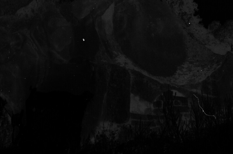
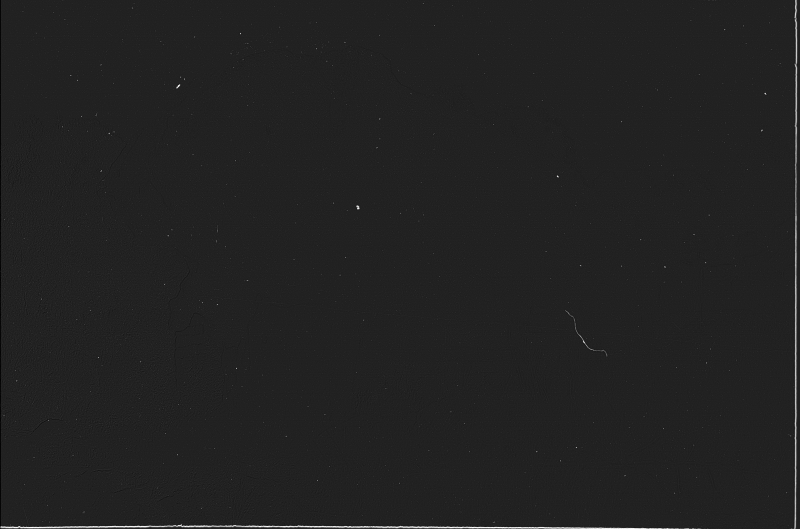
I don’t remember whether I mentioned it already or not, but anyway: my goal by removing the contribution of the visible image is to obtain a cleaner IR histogram which I can more easily threshold to isolate dust (black spots) and scratches (white streaks) from background. The first experiments I did with GIMP showed that it was often difficult to get all the dust without ending up selecting some parts of the image data bleeded into the IR image.

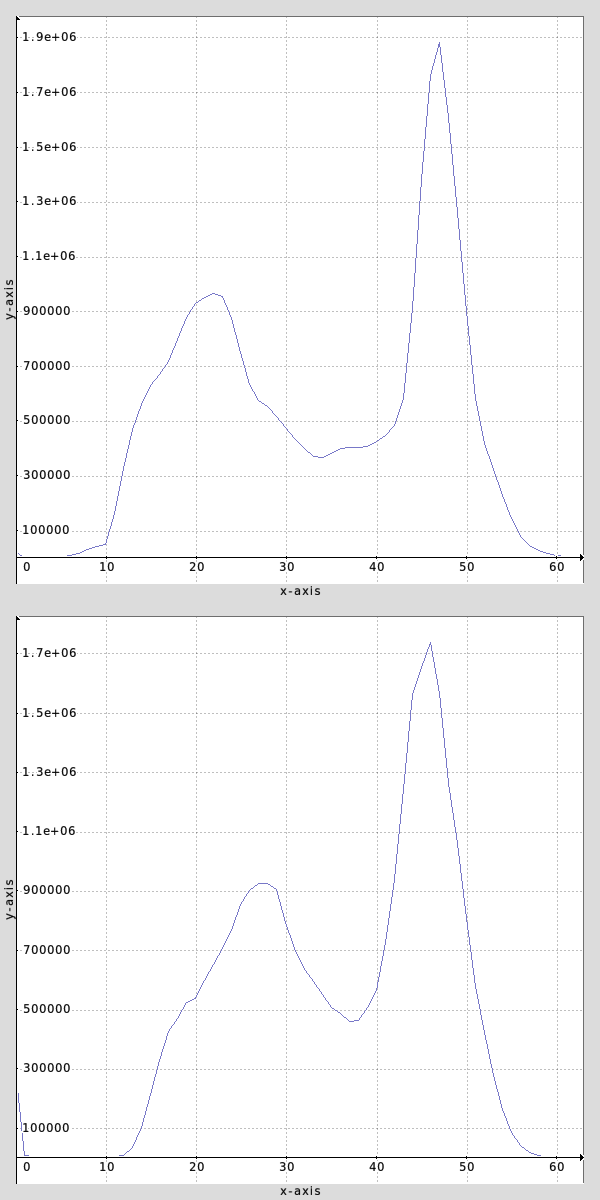
It shows how wide the histogram is if left as-is.

So my goal is not to completely clean it, I only need to increase signal/noise for a simpler threshold detection. Keep in mind that I don’t want to do it one by one manually… I am ready to visually check dust/scratches masks before inpainting, sure, but manual tuning should be kept to a minimum.

The subtraction of a smoothed copy is an idea already proposed, I just haven’t tested it yet.

Threshold by area? what do you mean? manually? I don’t want to

Can you elaborate about the “gamma” test you mentioned?

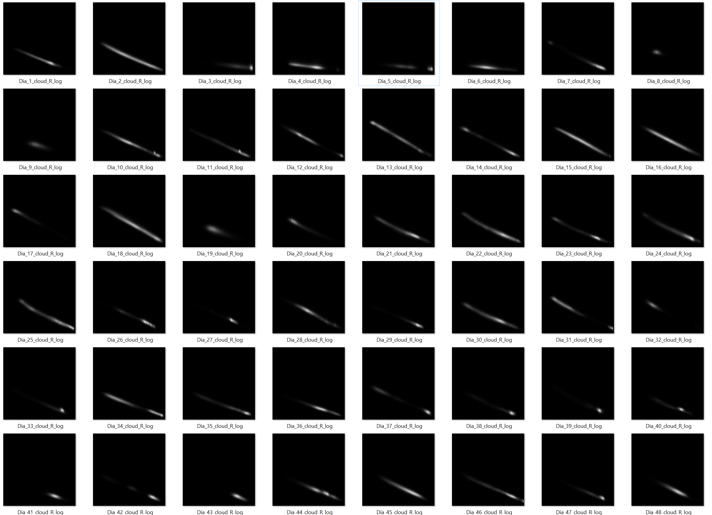
Also, for info: https://www.hpl.hp.com/techreports/2007/HPL-2007-20.pdf (which was already posted earlier). Given my point clouds I could use the data for interpolation, cutting out the leftmost, non-linear part of the curve. This way I would end up with a very linear correlation, easily removable. It will overestimate contribution in dark areas, but I think that is not an issue.

Jossie · December 7, 2021, 12:24pm

My assumption is, that the attenuation (in percent) for each pixel affected by dust/scratch is the same in IR as in the RGB-channels. Thus dividing by a normalized IR-image will remove the dust/scratch in the RGB image.

Hermann-Josef

garagecoder · December 7, 2021, 12:28pm

Thanks for the links, it looks interesting and I’ll need to do some reading. The quick gamma check I did in gmic is:
gmic Dia_10.tif k. n 0,255 negate apply_gamma 0.45

And here is a reduced crop of the output (I’m assuming you don’t mind me displaying it here):

The article about decorrelation says:
“The algorithm therefore assumes that in the density domain the contribution of the image forming dyes on the film to IR response is linear”

It looks as though your IR is quite correlated to the red channel by matching geometric mean:

But even then, it’s probably still better to variance smooth the IR (variance_patch 11 shows the marks quite clearly) and subtract.

garagecoder · December 7, 2021, 2:08pm

Using the red channel, I managed to get this far:

I cheated using some of my own filters in g’mic plus another to set geometric mean:
gmic Dia_10.tif k[0,-1] channels.. 0 set_mean 0.5 gcd_fmean_local 3,2 sub n 0,1 pow 3

set_mean : skip ${1=0.5},${2=0}
  if $2==-1
    m "_func : pow -1 sub 1" m "_finv : add 1 pow -1"
  elif $2==0
    m "_func : log" m "_finv : exp"
  elif $2==1
    m "_func : skip 0" m "_finv : skip 0"
  elif $2==2
    m "_func : sqr" m "_finv : sqrt"
  fi
  repeat $! l[$>]
    m={[im,iM]} n 0.002,0.998 ($1) _func *.. {i/ia#0} rm. _finv n $m
  endl done
  uncommand _func,_finv

olma · December 7, 2021, 2:49pm

Thanks, the result looks basically perfect.

I’ll take my time to decipher your script and I’ll try to apply it to my slides!

garagecoder · December 7, 2021, 3:10pm

No problem, there’s still a lot of work for you to do but it’s a start

Describing the above technique in words (with IR and red channel images):

Set both images geometric mean = 0.5
Square the values of each image
Divide each image by a gaussian filtered copy (small radius, may need to add an epsilon to avoid div by zero)
Square root values of each image
Subtract them (image difference)

For viewing only: normalize and apply exponent (a threshold won’t care about that anyway)

Explanation about the squaring: it makes it ~quadratic mean, but the ideal I think would be patch maximum, so you could use exp and log rather than sqr and sqrt, just be careful with value ranges…

Reptorian · December 7, 2021, 4:32pm

@garagecoder Just one little thing of note. Don’t use m,n as variable names. It would be easier to understand if they weren’t already names for command. That’s why in my G’MIC script, I avoid doing that.

garagecoder · December 7, 2021, 4:36pm

Yes sorry, you’re quite correct that’s some terrible code style! Normally I do try to avoid it, but haste got the better of me there.

alex666 · December 7, 2021, 8:51pm

Gimp resynthetizer is currently dead…
I pray that its resurrection will take place very soon.

olma · December 8, 2021, 9:59pm

I see it here: https://github.com/bootchk/resynthesizer
Last commit in May. I haven’t tried it though but it should work under GIMP 2.10

olma · December 8, 2021, 11:51pm

I realise now that density is a logarithmic transformation of the image values. I should scale accordingly X and Y in my correlations.

olma · December 13, 2021, 12:54pm

I haven’t yet studied in detail or tested the script by @garagecoder but I did a quick test with a log-linear scale (log red channel, linear IR).
The results are basically perfectly straight lines, therefore it should be very easy to remove the contribution by the visible light on the IR.

Check the results:

Script:

i ${1},0,2,2
crop 20%,20%,80%,80%
+channels[0] 0
log.
ap[1,2] "unroll x"
normalize[1,2] 0,1500
append[2] [1],y
pointcloud. 1
normalize 0,255
o[2] {0,b}_cloud_R_log.tif,uchar

The slope of the curves is also very similar, maybe it can be estimated from a whole roll so that even slides with few points, or points very similar in brightness, can get a good estimate.

After subtraction a threshold will likely be enough, or a more advanced approach like what was suggested earlier, and which I haven’t tried yet.

For info, I did the same with a more recent slide roll I know for sure was an E6 process, and which I know was not mixed up with other rolls.

The IR channels look very much alike and the log-lin graphs are basically identical, making definitely possible the calculation of a single linear regression for the whole roll.

garagecoder · December 13, 2021, 11:55pm

Yes, everything appears to be as described in the articles about IR/red channel. I think the next barrier could be noise; the match is much better in log space, but at such resolution the individual pixels aren’t likely to align. Downscaling might partially fix that. Here is the median transfer curve from indexed red channel log values to IR (red channel values shown in green, IR in red):

Perhaps the scratches will be separable enough anyway…

Neeman · January 3, 2022, 12:29am

For me, unfortunately, the correlation is not liniar (Nikon Coolscan ED 5000).

As both IR and Red channels are liniar (raw data from Vuescan), it also doesn’t make much sence to “log” red channel.

Attached are the translation curves from Red to IR for 3 differend negatives (1,2,3 - liniar) - (1r, 2r, 3r - Red channel Loged).

Untitled2384×1381 70.7 KB

I guess, it’s about different exposures (gain) per channel and a lot of underexposed area with noise on the left side of the curve.

I’ve tried different solution (RGBA tiff):
gmic.exe
1.tif
split[-1] c
rm[-2,-3] #keep only Red and Alpha channels
[-2] [-2] #copying both for further operations
crop[-1,-2] 5%,5%,95%,95% #cutting borders from copies
command andy_kelday gcd_mean_transfer_curve[-2,-1] #calculating the Red to IR transfer curve
rm[-2] #deleting copy of red channel
[-1] # copy of IR is replaced by GCD funcion, with transfer curve data - copying it
+resize[-1] 100%,0.15%,100%,100%,2 #averaging the curve (2) and making less points to a new position
crop[-3] 0,0,0,0 #getting the leftmost point of the curve
crop[-2] 0,100%,0,100% #getting the rightmost point of the curve
append[-3] [-1],y #these two lines merge the points of the curve
append[-3] [-2],y
rm[-1,-2] # removing temp data
split[-1] c # these three lines reallocate Y value of the curve to the same channel
append[-2] [-1],x
rm[-1]
apply_curve[-3] 1,{-1,^} # applying averaged transfer curve to original Red channel
rm[-1] # removing transfer curve, so only Transferred Red and IR uncut channels are left
sub[-1] [-2] # subtraction of transferred Red from IR

It provides quite good results.

Though I stuck with generating a clear defect map because of noise (it is a real barrier). I assume, some “credibility” mask should be applied as well (https://citeseerx.ist.psu.edu/viewdoc/download?doi=10.1.1.408.6190&rep=rep1&type=pdf).
However, I haven’t tried it, yet.

garagecoder · January 3, 2022, 1:03am

I’m pleasantly surprised to see the mean transfer command being used (I didn’t really “advertise” it)! I wonder then if the second version I have would be useful too (median transfer curve)… I’ll probably clean it up and push it some day soon.

Neeman · January 3, 2022, 1:06am

Thank you for it !!!
It saved my time

Neeman · January 5, 2022, 8:26pm

I’ve implemented an algorithm with Credibility factors from the article above.

Still playing with different credibility map sources / map generation formulas, trying to find a universal solution for all types of noise (Grayscale of original image seems to help with weak-moderate noise). Also I’m trying to find any information about “photometric functions” which can improve my implementation (article provides no specific examples of such functions).

As for non liniar Red channel cast to IR, after some tests it appeared, that “non liniar” correlation is specific to some film types. In my case it was Konica VX200-N.
Tried converting to CMY in order to uncast Cyan (as per article). However, IR to Cyan also wasn’t liniar. So far, no luck in finding a universal IR decorrelation solution… I believe IR channel for Konica VX200-N is affected by Green & Blue channels as well, not just Red. I’m about to give up for a while…

P.S. I wish I could have a look at the original Nikon’s ICE code

Neeman · January 10, 2022, 9:56pm

So, after a couple of test days:

decorrelation works best when both Red and IR channels are in Logarithmic domain. Converting liniar Reds and IRs to log domain provided best results for me.
- Olma, it seems, that IR channel in your files is already logarithmic
- Barriers: some sources even in Log domain has non-liniar correlation.
In case of liniar correlation, Red values can be “aligned” to IR channel, based on simple liniar regression
- Difference between two regression techniques - #5 by olma
- Barriers: when source is too dirty, mean level can be affected by IR exessive signal (threshold to IR, eliminating “defect” signal can help)
prepared Red channel is substructed from IR
then values are returned to liniar (by exp(x)) in case of liniar color space workflow (my case)
liniar [R], [G], [B] channels are divided by decorrelated liniar IR
- it restores luminance in some dirty but still transparent areas
- Barrier: although luminance is restored, regions are still slightly visible due to less noise (film grain ?) versus neigbouring areas
IR channel (and RGB channels if used) then copied for credibility map generation and made less detailed to average out the noise
- I used blur 2-4
Credibility map is built
- I’m still not sure about optimal combinations of contrast / bilateral / deviation functions and IR/Visible sources)
- information regarding Credibility maps can be found in HP article in previous posts
Credibility weighted algorythm is applied to IR low-detail channel to generate the mask
Thresshold is applied to generate the final mask
inpaint_pde is applied to hires image with generated mask

Quality still loses to original Nikon ICE, however now the result is much closer.

Main challenges for me now:

non-liniar IR-visible channels crosstalk (top priority)
- Mean transfer curve doesn’t work. Probaly some transformational 4x4 RGBI matrix/function should be calculated / applied.
grain / noise in restored areas (step 5 above), which were not covered by inpaint mask

olma · January 11, 2022, 7:39pm

Hi and thanks for the summary.

I have very little free time and I haven’t done anything since the last tests, but I’m happy to see you got that far.

When you think the scripts are usable you could post them to GitHub for everyone to see and provide feedback/improvements! It is a useful work which seems already good for many purposes.

Neeman · January 21, 2022, 10:37pm

So, my research from the last week:
there’re two main reasons of Infrared channel being affected by “ghosts”:

scanner generated channel’s crosstalk (due to poor isolation of frequencies, reflections, etc)
– almost not the case for professional scanners, however may happen in cheaper models
scanned materials’ specifics (even more relevant for negatives).
– in my case, Cyan dye of Konica VX200 was responsive to infrared day light and was opaque to IR light of scanner / behaves in IR light just as in visible spectrum…
– in the worst cases (i.e. overexposed bright window) some areas can be even more opaque, than scratches - thresholds or decorrelations may minimize the effect but cannot separate scratches completely (it is not the matter of domain - liniar, log, density, root or any other.)

As for simple cases, where the scratches are still more opaque to IR than cross signal from Red, liniar regression works well. And i’ve tested successfully an algorythm which helps to better auto align Red to IR “ghost”:

crop image from borders
unroll IR and Red x-wise
regress Red to IR
subtract regressed Red from IR and make values absolute
sort the IR and Red pixels by the result of step 4
– I’ve used pixelsort[IR, RED] +,x,[SUB]
cut the tail pixels of step 5 from the Red and IR channels (I’ve tried it with 2-5% cut steps)
– the bigger value pixel has in step 4, the furter is the pixel from the expected signal, the more likely it stands for the scratch / negatively affects the regression coefficients, thus excluded
revert to step 3 with modified (cut) Red and IR channels / repeat 10-30 times
in the end you receive “ideal” A and B coefficients, which you can apply to original Red and subtract it from original IR

So this approach step by step excludes noise and scratches information to ensure better alignment of Red and IR orginal signals / crosstalk.

Sorry, I cannot publish the code at the moment, as it’s too dirty and I have no time to clean it (studying non-liniar regressions…)
– I’ll leave it here as is, just in case someone searches this information (as I was searching a week ago )…