Scanned image scratch removal with “ICE”

chris · March 3, 2020, 11:18pm

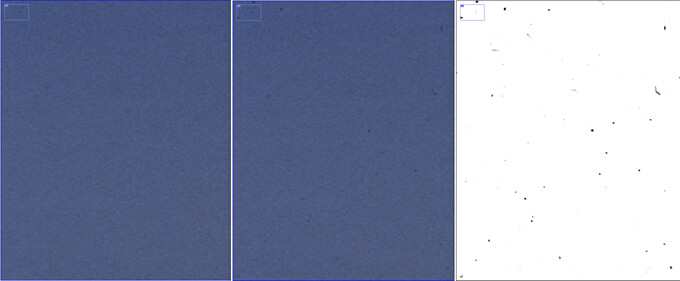
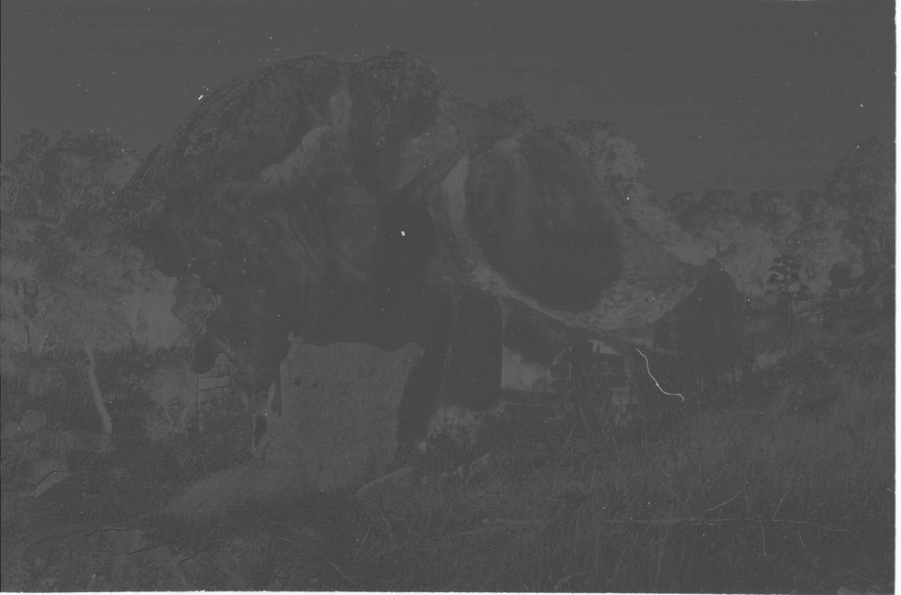
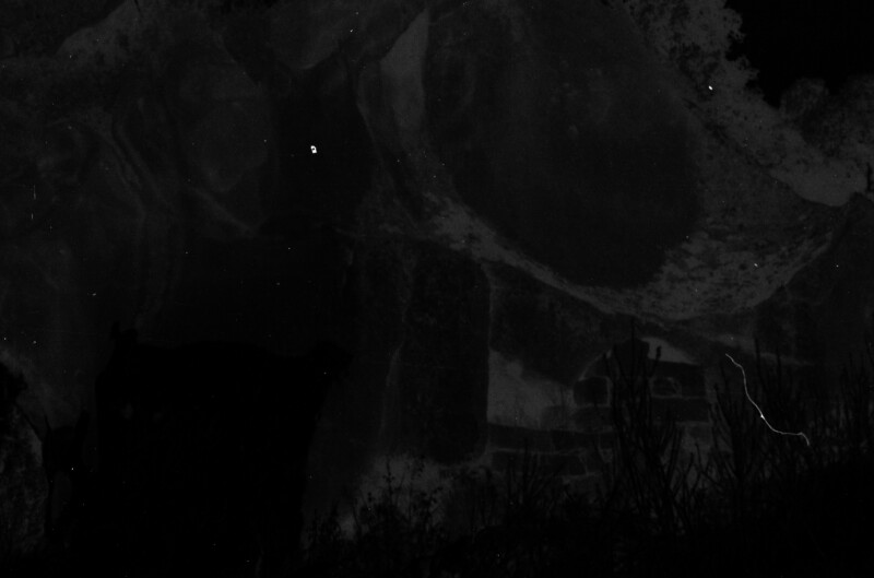
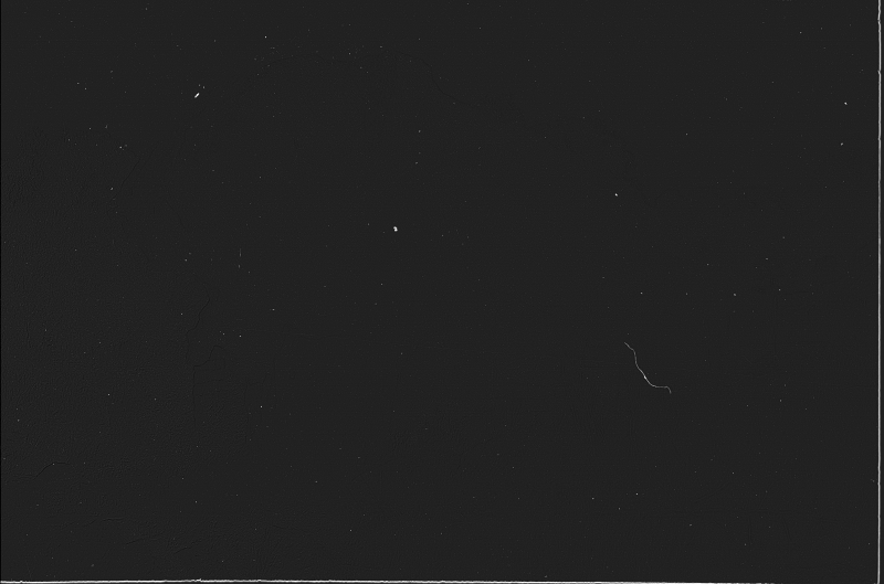
As I cannot edit my old post (@paperdigits, @patdavid, could you maybe reenable editing on this topic such that I can update it and make the files available again?), please find here a new scan of the original image if you want to test scratch removal. For a reasonable size, it’s only a cut-out of the original image, but it shows several kind of issues to test scratch removal again, especially a “telegraphy line” (horizontal line over the whole image) and some dust spots of different size.

example.tif (9.7 MB)
(3600 dpi scan on Reflecta CrystalScan 7200 with VueScan, saved as “raw” tiff file)

If you are interested, I can make the whole file available again (approx. 150 MB), and I even have a 7200 dpi scan available now (approx. 600 MB), but it would be good if this could be a permanent solution this time (maybe directly on pixls.us, e.g. as part of raw.pixls.us?).

paperdigits · March 4, 2020, 12:12am

I’m on mobile right now, but your post doesn’t look locked to me.

afre · March 4, 2020, 4:51am

I cannot edit my old OPs either (or old posts in general). I think only mods can do that. Would be useful especially for threads that have 100+ replies.

olma · December 6, 2021, 1:57pm

Hi, thanks for the feedback.
Can you link or share the ImageJ script? I’m interested in testing it.

Jossie · December 6, 2021, 3:24pm

@olma Currently the script is not working. I did some “upgrade” to it (not related to scratch removal) and there is a bug somewhere I have to find.

As I explained above its median filtering the IR and subtract it from original IR, thresholding and smoothing the difference image. That is all, using genuine imageJ commands. Then I replace the IR-image in the scan file by this manipulated IR-channel and process this with SilverFast iSRD.

In the meantime (since my last post) I tried a procedure relying on the assumption that the reduction of the signal due to dust/scratch is the same for IR and RGB:
Threshold the IR-image, normalize it and then divide the RGB-image by this (my previous assumption of subtraction was wrong). Here is a demo of what I got with this procedure:
grafik
Left: corrected, center: original, right: IR-channel
Of course this won’t work for Kodachrome since the scene is readily imaged in the IR-channel.
Problem is the slight difference in image scale between IR and RGB. Currently I have no idea how to correct this.

Hermann-Josef

olma · December 6, 2021, 11:10pm

I tried to check correlation between R, G, B, grayscale and IR channel, hoping to find something which could help me subtract better the image data leaked to the IR channel.

I run this script:

#load color and IR, no preview
i ${1},0,2,2
#cut out black borders
crop 20%,20%,80%,80%
div 257
+channels[0] 0
+channels[0] 1
+channels[0] 2
+rgb2srgb[0] luminance. srgb2rgb.
ap[1-5] "unroll x"
append[2] [1],y
append[3] [1],y
append[4] [1],y
append[5] [1],y
ap[2-5] "pointcloud 0,256,256"
ap[2-5] "-normalize 0,255"
o[2] {0,b}_cloud_R.tif,uchar
o[3] {0,b}_cloud_G.tif,uchar
o[4] {0,b}_cloud_B.tif,uchar
o[5] {0,b}_cloud_mono.tif,uchar"
rm

So what you get is on X axis the value of R, G,B,grayscale and on the Y axis the value of the IR channel. I have to point out that the grayscale is the “luminance”, which almost discards the blue channel, but it doesn’t matter much: the channels are not so different.

The stronger the leak, the more grouped together the values are.
Darker images have more points on the left, brighter ones more points on the right.

The results are best shown using the Windows thumbnails (each photo is followed by R, G, B, grayscale point clouds):

Overall, reddish photos work best with red channel, blue photos with blue channel and so on, so the grayscale is the best option.

I would be curious to see the same applied to Kodachrome to see how the clouds lok like!

But also the baseline is not a line, and a linear correlation would not work to remove effectively the leak. It is often good enough, but some photos have a noticeable curve.

At this point for my E6 slides I’m not sure how to proceed about subtraction of the leak.

I will try the blur as you suggested, at least to compare.

Jossie · December 7, 2021, 8:11am

As far as I can see for E-6 there is hardly any signal from the scene in IR. So I normalized the IR to the average level, put a threshold to avoid introducing noise and then divided every channel by this modified IR-image. No smoothing applied here. That was the example above.

Smoothing was applied by my imageJ macro in preparation for the application of iSRD in SilverFast only. It was meant to slightly enlarge the defects to avoid halos around the defects if iSRD is applied with a minimum detection setting.

Hermann-Josef

garagecoder · December 7, 2021, 9:10am

Hi, would you perhaps be able to share here a complete original image which demonstrates the correlated IR channel problem? Ideally with some scratches too.

olma · December 7, 2021, 9:26am

I’m not sure I understand the point of dividing the channels by the normalised IR image.
Can you elaborate a bit? how does it work? the result of the division is the final clean image?

Back to my films: maybe they were not all E6, I’m not sure: I’m working right now on slides from my parents, but I remember mixing them up as kid so some rolls could even be Kodachrome! The film is now many km away from me and I cannot check. So you may be right and I’m actually working on a script which will be good for Kodachrome.

See an example of what I have also on rolls which I know for sure are E6:

Back to the previous experiment, I made a mistake: I used “binary” mode of pointcloud which doesn’t give a proper idea of the clouds.

I repeated with type “1 accumulation” and I got much more reasonable correlation between channels and IR:

Now the red channel is always the one with the best correlation (sharper and longer cloud).

I can work from here, but I’m not sure when I’ll have time. First I have to think about the algorithm.

olma · December 7, 2021, 9:37am

I put here some examples (original, IR only, point clouds) with strong and weak bleeding.

I cannot say how long I will keep the folder, but likely a year at least.

Also, here the corrected script:

i ${1},0,2,2
+crop 20%,20%,80%,80%
rm[0,1]
+channels[0] 0
+channels[0] 1
+channels[0] 2
+compose_channels[0] + div. 3
# scaling to get a 1500 pixel final cloud
div 45
ap[1-5] "unroll x"
append[2] [1],y
append[3] [1],y
append[4] [1],y
append[5] [1],y
ap[2-5] "pointcloud 1,1500,1500"
ap[2-5] "-normalize 0,255"
parallel "o[2] {0,b}_cloud_R.tif,uchar","o[3] {0,b}_cloud_G.tif,uchar","o[4] {0,b}_cloud_B.tif,uchar","o[5] {0,b}_cloud_Z_mono.tif,uchar"
rm

If anyone has Kodachrome, please post an example (color, IR, clouds). I’m not sure I ever saw one.

garagecoder · December 7, 2021, 9:48am

Thanks for those, it makes it much easier to understand your purpose!

P.S I think you should be able to attach an “original” 4 channel tif on here directly, if you prefer.

olma · December 7, 2021, 10:05am

It’s 250 MB…
I could crop it of course, but I think it would not be the same.
I think that the IR image posted earlier is enough to understand.
Anyone interested in replicating likely would have some on their own.

garagecoder · December 7, 2021, 10:58am

I’m not sure if much can be gained by attempting to remove the image contribution to the IR, since as you say it’s a non-linear combination. One approach is to focus only on improving the separation of scratches within the IR layer. I suggest three things for that:

subtract/divide a locally smoothed copy (median, bilateral etc.)
threshold the scratches you want removed by area
threshold the final by value

By that point anything included which is not a scratch would cause imperceptible changes with inpainting anyway.

Edit: a simple exponent (“gamma”) on the negative IR can reveal the scratches well to the eye, so I think there’s enough separation to work with.

olma · December 7, 2021, 12:10pm

First of all thanks for your contribution.

I don’t remember whether I mentioned it already or not, but anyway: my goal by removing the contribution of the visible image is to obtain a cleaner IR histogram which I can more easily threshold to isolate dust (black spots) and scratches (white streaks) from background. The first experiments I did with GIMP showed that it was often difficult to get all the dust without ending up selecting some parts of the image data bleeded into the IR image.

It shows how wide the histogram is if left as-is.

So my goal is not to completely clean it, I only need to increase signal/noise for a simpler threshold detection. Keep in mind that I don’t want to do it one by one manually… I am ready to visually check dust/scratches masks before inpainting, sure, but manual tuning should be kept to a minimum.

The subtraction of a smoothed copy is an idea already proposed, I just haven’t tested it yet.

Threshold by area? what do you mean? manually? I don’t want to

Can you elaborate about the “gamma” test you mentioned?

Also, for info: https://www.hpl.hp.com/techreports/2007/HPL-2007-20.pdf (which was already posted earlier). Given my point clouds I could use the data for interpolation, cutting out the leftmost, non-linear part of the curve. This way I would end up with a very linear correlation, easily removable. It will overestimate contribution in dark areas, but I think that is not an issue.

Jossie · December 7, 2021, 12:24pm

My assumption is, that the attenuation (in percent) for each pixel affected by dust/scratch is the same in IR as in the RGB-channels. Thus dividing by a normalized IR-image will remove the dust/scratch in the RGB image.

Hermann-Josef

garagecoder · December 7, 2021, 12:28pm

Thanks for the links, it looks interesting and I’ll need to do some reading. The quick gamma check I did in gmic is:
gmic Dia_10.tif k. n 0,255 negate apply_gamma 0.45

And here is a reduced crop of the output (I’m assuming you don’t mind me displaying it here):

The article about decorrelation says:
“The algorithm therefore assumes that in the density domain the contribution of the image forming dyes on the film to IR response is linear”

It looks as though your IR is quite correlated to the red channel by matching geometric mean:

But even then, it’s probably still better to variance smooth the IR (variance_patch 11 shows the marks quite clearly) and subtract.

garagecoder · December 7, 2021, 2:08pm

Using the red channel, I managed to get this far:

I cheated using some of my own filters in g’mic plus another to set geometric mean:
gmic Dia_10.tif k[0,-1] channels.. 0 set_mean 0.5 gcd_fmean_local 3,2 sub n 0,1 pow 3

set_mean : skip ${1=0.5},${2=0}
  if $2==-1
    m "_func : pow -1 sub 1" m "_finv : add 1 pow -1"
  elif $2==0
    m "_func : log" m "_finv : exp"
  elif $2==1
    m "_func : skip 0" m "_finv : skip 0"
  elif $2==2
    m "_func : sqr" m "_finv : sqrt"
  fi
  repeat $! l[$>]
    m={[im,iM]} n 0.002,0.998 ($1) _func *.. {i/ia#0} rm. _finv n $m
  endl done
  uncommand _func,_finv

olma · December 7, 2021, 2:49pm

Thanks, the result looks basically perfect.

I’ll take my time to decipher your script and I’ll try to apply it to my slides!

garagecoder · December 7, 2021, 3:10pm

No problem, there’s still a lot of work for you to do but it’s a start

Describing the above technique in words (with IR and red channel images):

Set both images geometric mean = 0.5
Square the values of each image
Divide each image by a gaussian filtered copy (small radius, may need to add an epsilon to avoid div by zero)
Square root values of each image
Subtract them (image difference)

For viewing only: normalize and apply exponent (a threshold won’t care about that anyway)

Explanation about the squaring: it makes it ~quadratic mean, but the ideal I think would be patch maximum, so you could use exp and log rather than sqr and sqrt, just be careful with value ranges…

Reptorian · December 7, 2021, 4:32pm

@garagecoder Just one little thing of note. Don’t use m,n as variable names. It would be easier to understand if they weren’t already names for command. That’s why in my G’MIC script, I avoid doing that.