Spectral film simulations from scratch

mikae1 · February 26, 2025, 9:10pm

I very much share your excitement! I sent early fan PMs to @arctic after watching his cryptic PlayRaw contributions for months. This example really caught my eye in May.

Sadly, I haven’t been successful getting it to run on my Fedora based Aurora installation using pip yet, so for now I just wait for your posts in this thread. Saw a recommendation for uv. Hope to try that this weekend! Perhaps your vkdt implementation can make it more accessible to Python imbeciles like me.

Yes, the roll-off looks insanely good in many of the examples I’ve seen. And regarding the colors… We shouldn’t forget that Kodak spent a century perfecting their colors. Their aim was not only to have an accurate rendition of colors, but also an eye pleasing one.

I genuinely do not think that the excitement for film is based on pure hype or trend. Of course there’s also the element of physically, but people spend an inordinate amount of time trying to achieve a proper film colors in Lightroom only finish it off with Adobe’s monochrome grain…

It kind of surprises me that after ~19 years of Lightroom and ~15 years of darktable, we’re still stuck with monochrome grain for color images and no attempts at replicating the other properties of film (like halation). Meanwhile the cine graders get all the shiny toys. There’s Filmbox and Dehancer and DaVinci Resolve recently got an amazing native Film Look Creator. The aim of the Film Look Creator is not to simulate any specific film, but to give film-like results with lots of control. In many ways it looks quite similar to what I’m seeing in this thread.

After some years of using darktable I’m somewhat OK with the tools I have at hand. I have, for the past 12 years I’ve used workflows that try to mimic a Portra 400 NC or VC look digitally, previously in Lightroom with VSCO presets/profiles and now in darktable with G’MIC sRGB Cube LUT.

It does not replicate the subtleties of film like what I’m seeing in @arctic’s PlayRaw examples though.

If @arctic’s filmsim comes to open source software I think we could expect some proper excitement for open source alternatives to Adobe’s products. There’s really nothing like it in the stills software world and still the demand seems huge.

This is an interesting observation. As I said earlier in this thread it’s a great way of making upsampling/interpolation artifacts vanish. We partially judge the sharpness of the underlying image based on the sharpness of the “grain layer”.

arctic · February 27, 2025, 12:30am

Yeah, sorry about that, this is really a minimal one-file gui solution that kinda works. You can try to match your monitor/os profile with the output profile of the sim. @NateWeatherly above in the thread was talking about having DisplayP3 as an ok solution to work with a ok color managed preview. Try to have a look into that! Here is the link to the post:

Also I am not super keen at having this as a final solution. I think there are much better human interfaces in other softwares (vkdt, darktable, rawtherapee, art…), so there is probably no need to rebuild everything. I see this as a tech demo that I am very comfortable at hacking, and go crazy with details. If it is going to be a viable solution for actual doing some work I could put together something better in the future. For now my focus has been the engine and the “look”. But thank you for the critic! It is in my mind.

arctic · February 27, 2025, 12:41am

I am jawdropped, even if it is a simplified version …3 ms is probably close to 4 orders of magnitude faster of what it takes in my hacky python for just grain generation.

I absolutely agree on this, I love the idea of upscaling and adding grain. And not being able to see the pixels when looking closer! Usually pixel-peeper is used with a negative connotation, but I guess grain-peeper only has a hipster positive aura.

He he, I think it looks already extremely good! If you need a bit of background on my assumptions about the grain model I will write something. If it helps!

I am also guilty of this, sometimes I wanted to work on it, but I just got sidetracked to try endlessly on random pics.

The way I create the filter neutral values is to fit a sigle gray pixel ([0.184,0.184,0.184]) in the input to obtain the same gray value as output (I actually fit Y filter, M filter, and print exposure). I find the filter neutral values quite sensitive to the pipeline, so not sure they will hold exactly. If they do that would be amazing.

I had a quick look to the code, and I am honored to see this effort, I will try to understand more. And I will try to run it on my desktop, with GPU, that is just taking dust lately.

olliwa · February 27, 2025, 1:32am

works on win11 too
just unzip last release
just two corrections to create filmsim.lut

pip install -r requirements.txt
...
cd agx_emulsion/data/profiles

arctic · February 27, 2025, 1:59am

Great comment @mikae1! If you need any help with the python part let me know.

I 100% agree here, and I hope to dig more and try to understand what are the general criteria in the spectroscopical data that encodes that, for now it feels something intangible, but there might be some way to rationalize at least partially what is going on.

Having a general tool not really dependent on ununderstood knowledge baked in the spectroscopical data sounds super cool!

Just for fun I made a comparison with some images I found on my computer from the playraw you referenced, all using the same underlying data. I processed it a few times over the last months, at different stages. They are edited independently (color balance do not exactly match), but I think they illustrate quite well the evolution of the sim.

In order:
(a) original play raw submission
(b) addition of more refined masking couplers
(c) early version of dir couplers
(d) the current default output of the large-color-gamut branch, from (c) we got new more effective dir couplers, plus new hanatos’s spectral upsampling (and much more stuff). Only negative/print exposure changed from default.
All with Kodak Portra 400 and Kodak Ektacolor Edge.

And oh man… I also have to say again that I am amazed by the subtle but satisfying changes the large color gamut input is bringing to the table.

Since I cannot get enough, here is another comparison shot from signatureedits.com, with everything default (Kodak Gold and Supra Endura). Input in 32bit linear ProPhoto RGB.

(left) darktable basic edit, (center) mallett2019, (right) hanatos2025

Even trying to match the two film sim better, i.e. with the enlarger filters, I cannot really get them feeling the same. The darktable ultra basic edit is with same white balance, using sigmoid with contrast 2, and color balance rgb with 30% global vibrance.

arctic · February 27, 2025, 3:21am

Uh interesting! I tried to have a quick look on scholar but no luck.
I found this generic data from the books I have. And indeed it seems to be pretty wide, especially red-blue sides.

From: The manual of photography photographic and digital imaging (ninth edition), Ralph Jacobson, Sidney Ray, Focal Press, 2000, page 388-390.

This is also quite interesting, haven’t tried to input images just for printing, or in any other middle step of the pipeline. It should not be too difficult, I guess I could interpret the linear RGB values as effective exposure of the print paper and compute everything from there.

hanatos · February 27, 2025, 10:22am

yeah we should probably discuss this some. for now i’m just considering “a lot” of grains inside one pixel, such that the spatial white noise distribution characteristics turn into some gaussian filtered white noise (a bit more blue). this is like the non-uniformity of grain numbers as seen through each pixel. now really i’d like to use some binomial/poisson random variate with expectation = developed density to sample which of these grains turn. whatever i did was probably wrong because it just floods the whole image with exorbitant amounts of noise. there’s something fundamentally awkward about the poisson distribution that i can never quite find intuitive… this fact that every particle brings their own variance… so more photons per pixel mean more variance. quite the opposite of a monte carlo estimator! anyways the number of developed grains per pixel is for now just directly the expectation n\cdot p.

right. i suppose the differences are subtle but probably exist (i use pretty crude approximations of the YMC filters for instance). i have nelder mead/adam optimisers in vkdt that are in theory able to wrap around a processing graph and fit module parameters to picked colours/loss module output. will try that fitting step and see what happens.

oh one more thing: i don’t use the envelope function. i figured the pipeline does not fluoresce, i.e. the wavelengths don’t exchange energy (other than projecting to cmy/rgb densities in between). in the very end, the scanning step projects to the 1931 CMF which already have the falloff at 400 and 700 nm just like the assumptions of the upsampling routine would be. would you have a particular image and settings for me that showed the cyan issue? i’d like to try and reproduce…

PhotoPhysicsGuy · February 27, 2025, 11:07am

Great! It really looks like those gamuts really exceed the sRGB gamut. I am also not claiming that “bigger-gamut = better” but that one has to keep this in mind wrt adjusting DIR-coupler settings.

hanatos · February 27, 2025, 1:56pm

looking at the couplers and the non local part again. maybe you can explain to me in simple non-python terms what this code is supposed to do

it interpolates quite a bit of stuff going back and forth between exposures and densities, and i’m lost.

from what i understand, a 3x3 coupler matrix is constructed, and applied to the (normalised, potentially exposure shifted) density curves by component wise multiplication to the 3 curves. why normalised? isn’t the matrix multiply without normalisation the same? normalisation just for the exposure shift in case it’s non-zero?

then why can you just subtract the result (isn’t that a density?) from the log exposure? and why go from this log exposure to density again? then from density to log_raw_correction? and why linear filter/gauss blur the log exposure correction? shouldn’t we blur linear scene referred light values instead? i assume the radius can be quite large here. and then finally the corrected/blurred log raw is going to density again, via corrected density curves.

this feels like going in circles a fair bit, potentially because it’s easy to write this in python? what’s happening conceptually here?

arctic · February 27, 2025, 2:39pm

The assumption behind the grain is that each layer has a total area coverable by particles proportional to the density max. Each sub-layer has thus a fraction of this area.
I am using a compound “binomial(poisson, p)”. Poisson for the xy point process of the particles across the planes, i.e. how many particles end up in each pixel bucket. Binomial for the probability of development (p), i.e. proportional to density/density_max. In reality the particles are not really random across the surface, so I added a simple saturation model to take into account the packing, i.e. reduced variance compared to poisson because occlusion. I do this by faking a larger amount of particles that reduces the relative variance, and by scaling the density at the end.

There is a smaller complication about fog. There is a density minimum that is always developed even without light exposure and we need to take that into account.

By the way, I made some code with numba that compute approximations of binomial and poisson, and might be closer to your implementation. Essentially I am using a set of approximation to compute the random numbers in different regimes. E.g. for binomial, from direct bernulli sampling to normal. In agx_emulsion/utils/fast_stats.py in the large-color-gamut branch, possibly useful.

This is the behavior of a single layer.

Minimal grain code for one layer, for making also the RMS figure.

import scipy
import numpy as np
import matplotlib.pyplot as plt

poisson_rvs = scipy.stats.poisson.rvs
binomial_rvs = scipy.stats.binom.rvs
# beta_rvs = scipy.stats.beta.rvs
n_particles = 1000 # on average per pixel
dmax = 1.0
od_particle = dmax/n_particles

samples = 1000
le = np.linspace(-3, 3, 512) # log exposure
p = scipy.stats.norm.cdf(le) # simple density curve
p = np.tile(p, (samples, 1))

samples_sat = []
uniformity = [0.5, 0.7, 0.9, 0.95]
for i, uni in enumerate(uniformity):
    saturation = 1 - p*uni*(1-1e-6)
    samples_sat_max = poisson_rvs(n_particles/saturation, size=p.shape)
    samples_sat.append(binomial_rvs(samples_sat_max, p)*saturation*od_particle)

seeds = poisson_rvs(n_particles, size=p.shape)
samples_binom_poisson = binomial_rvs(seeds, p)*od_particle
samples_binom = binomial_rvs(n_particles, p)*od_particle # case of perfect ordering
# samples_beta = beta_rvs(p*(n_particles-1), (1-p)*(n_particles-1), size=p.shape)*n_particles*od_particle

plt.plot(le, np.std(samples_binom_poisson, axis=0), label='Binomial(Poisson)')
plt.plot(le, np.std(samples_sat[0], axis=0), label='Binomial(Poisson) with uniformity=0.5')
plt.plot(le, np.std(samples_sat[1], axis=0), label='Binomial(Poisson) with uniformity=0.7')
plt.plot(le, np.std(samples_sat[2], axis=0), label='Binomial(Poisson) with uniformity=0.9')
plt.plot(le, np.std(samples_sat[3], axis=0), label='Binomial(Poisson) with uniformity=0.95')
plt.plot(le, np.std(samples_binom, axis=0), label='Binomial')
# plt.plot(le, np.std(samples_beta, axis=0))
plt.xlabel('Log Exposure')
plt.ylabel('RMS Granularity')
plt.legend()

I didn’t understand this comment about the envelope. What is this envelope in this context?

For sure this test image I created shows the issue.
gradient_hdr_rgb.exr (390.8 KB)
You can import it both in linear Rec2020 or linear ProPhoto RGB.
(left) interpreted as linear Rec2020, (right) interpreted as linear ProPhoto RGB

The output is still smooth in a large output color space, so for some reason we are hitting the clipping of the output sRGB hard on the cyan side.

Like shown before already in these tests. But why this is happening and if it is expected behaviour of prints it is a different topic. The nice thing is that I don’t remember I have encountered any real world image that I processed in which this was a disturbing issue.
As @PhotoPhysicsGuy was commenting, by looking at real data, the gamut of print papers is quite large and extends beyond sRGB, also on the cyan side.

hanatos · February 27, 2025, 2:56pm

ah i meant the band pass envelope function in this image above, explicitly cutting off extreme wavelengths:

arctic · February 27, 2025, 3:10pm

Indeed there is no fluorescence/phosphorescence, but from my experience there are unpleasant colors, especially reds, when film sensitivities are broader than CIE 1931 CMFs. And there are less of this issues when sensitivities are more spectrally narrow in the visible. So it is not really related to the input-output spectral bounds, but to the way film sees light. I can provide some more examples to support the improvement. But I am also ok to be disproven.

I will answer later on the couplers, I like the confusion in your comment, it explains perfectly the acrobatics in the code. Trust me, in my mind and notes there is some rationale. But it might crumble after a revision by someone else. I’ll try to explain.

hanatos · February 27, 2025, 6:15pm

no pressure, no rush! i’m just getting carried away here… will look at grain again in the meantime.

i did the ym filter fitting now btw. i had to fit cyan too, but even then some combinations of film and paper turn to negative filter percentages… not very reassuring. this is matching 0.184 input to 0.5*D50 on the output… sometimes i can get more pleasing skin tones (with positive filter weights) when trying to match that directly. anyways, continues to be good fun!

arctic · February 27, 2025, 10:01pm

No worries no pressure
I tried to write down the reasoning, but it is probably more convoluted that I thought. Anyway here is an explanation attempt of my inspiration, trying to justify the steps.

DIR couplers are chemicals released together with the formation of (coupled with) density and inhibits the development of more density. They diffuse spatially, typically 10-15 micrometers (I don’t a a reference for this for now, just a reasonable guess), one layer is 2-5 micrometer. So they diffuse both across layers and in the image plane. These are very small distances, a bit larger distances than the grain. For reference typical PSFs for sharp lenses are 2-3 micrometers, 5+ for worse ones.

It would be nice to make a small kinetic scheme to simulate proper inhibition kinetics, and integrate the differential equations, but it would be quite computationally expensive I think.

My drastic assumption and reasoning are:

wathever we do we want to respect the density_curves data. They are measured exposing with a neutral illumination the film (d55 or d65), creating density in all layers simultaneously.
the density is a measure of concentration of developed dyes (Lambert-Beer law). Since the proportionality density-concentration depends by the absorption efficiency, I normalized by max_density to have a 0-1 quantity of dye comparable in every layer.
I am first assuming that density_cmy_0 computed with the original density_curves is a first estimate of the density that would form on the layer.
I now assume that the quantity of DIR couplers generated on a layer is proportional to density_cmy_0 normalized, because they are formed in a coupled way during development. This is of course an approximation.
the couplers diffuses across the layers and in space, i.e. gaussian blurring.
next I am assuming that the development of film and the quantity of density reached in a layer is kinetically controlled given a certain time of development. Thus the density produced on a layer is “velocity of development x time of development” (at least when far from density max). Time of development is fixed. While velocity of development can change with inhibition.
I am assuming log exposure to be proportional to the velocity of the reaction of the development process (density created per second). Light produces Ag centers, that will speed up the reaction of silver halides + developer → silver (and later → dyes). Locally more density is generated if more Ag centers were created by light. We can further assume that log_raw (from the toe intersection) is linear to the amount of Ag centers (or particle with at least an Ag center that can be developed). Within this assumption log_raw is a measure of quantity of stuff (latent particles). This is of course another simplification.
inhibitors slows down locally the development, causing less halide to silver conversion. We can think as inhibitors able to subtract/inhibit Ag centers, i.e. virtually reducing log exposure (log_raw). So log_raw_corrected is computed as log_raw - the quantity of inhibitors present in that layer and position.
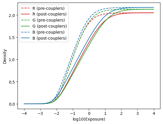
If we would stop here and reinterpolate log_raw_corrected with the normal density_curves we would reduce the contrast, and our simulation would not match anymore the data. To fix this we can generate a new set of virtual density curves like if inhibitors were not active: density_curves_0. These curves are more contrasty, and they give exactly density_curves after the inhibitors are applied with neutral illumination to the film. Now our film respect the original data, and the midtones will be essentially unchanged. Saturated colors instead will have less density on the channels with already low density.

Of course we need to make sure that the amount of inhibitors is calibrated to have a reasonable effect. The reason we can subtract log_raw with inhibitors coming from normalized density is then this assumption that both things can be interpreted as quantity of stuff (Ag centers/particles with Ag centers and chemicals suppressing Ag centers).

The spatial xy effect of the dir couplers is to increase sharpness. And we apply a blur to couplers amount (coming from density) because we are interpreting them as quantity of stuff moving around.

This is an example of density curves:

With dir_couplers_amount = 1.0 we get this amount of couplers in the layers:

Green in the middle of the stack receives from two sides.

This is the coupler matrix illustrating the amount of DIR couplers diffused in each layer from the starting one:

And these are density curves pre and post appling couplers. Density curves pre-couplers (dashed) are virtual, never really happening on the film:

This description might have scientifically unsound bits, and I can probably refine the assumptions to be more correct in the formulations. I think anyway that the final algorithm is a sort of simplest possible one able to produce the inhibition. We can for sure make it more complex and more true to reality.

arctic · February 27, 2025, 10:05pm

Wow great that you can fit filters on the fly. This opens up also the possibility of more drastic changes to the profiles without the fear of loosing a trusted neutral point for the filters.

Print paper sensitivities are calibrated to work with filtered tungsten light going through typical negatives. Negative filters is probably a sign that things are a bit uncalibrated compared to reality. In the real world everything should be possible with touching the cyan filter much, too.

I wonder why 0.5 * D50 and not 0.184 * D50 and if it matters.

hanatos · February 28, 2025, 1:30pm

excellent, thank you. now if i use 1000 grains per pixel and a binomial on top of my filtered fake poisson i think it starts to look much better. the binomial resolves some of the overly blue noise regular look. i may think about the saturation part again, didn’t model this yet.

apparenly it’s just very sensitive to the YMC filters. i replaced these with some smoother version and re-ran the fit, now everything is positive in [0,1] as expected. i would still say that i have some yellow cast issue with the kodak supra|portra endura . maybe that’s my crude filter approximation still.

ah i was thinking because it’s a display transform … but you’re right gamma will go on top after that. let me re-run with 0.184 and see what happens.

(thinking about the couplers…)

Jiyone · February 28, 2025, 5:11pm

I wonder if you will add anytime soon some black and white film and B&W paper, with the ilford multi-grade having different layers with different density.

nosle · February 28, 2025, 10:21pm

In addition to @Jiyone question above, how complicated is it to add further sims? Is the data for making more available,?

Does anyone know how different the nc portras were to the newer prefix less versions?

mikae1 · February 28, 2025, 10:36pm

Here I guess:

mikae1 · February 28, 2025, 10:39pm

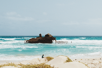
Yes, looks good indeed! I get stuck on the “greenery” in the lower edge of the picture. Also the ship wreck shadows. It looks so distinctly filmic (and not in the filmic rgb sense ).

What’s your take on mallett2019 vs. hanatos2025? I’ve been on the road and judging comparisons from my phone display, but I believe I prefer hanatos2025 in almost every case.

Yeah, made me think about what you said somewhere earlier in the thread about not being based on measurements but technical documents. Also, I guess at some point the films will have to be named a bit differently. Godak Bortra?