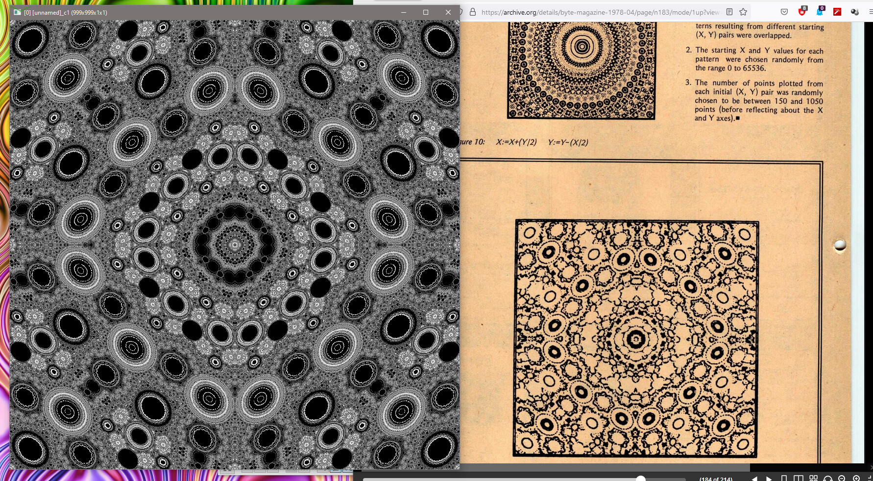
Awesome! Just when I had managed to reproduce @David_Tschumperle’s result using Julia:
Awesome! Just when I had managed to reproduce @David_Tschumperle’s result using Julia:
I’m interested, how the Julia code looks like?
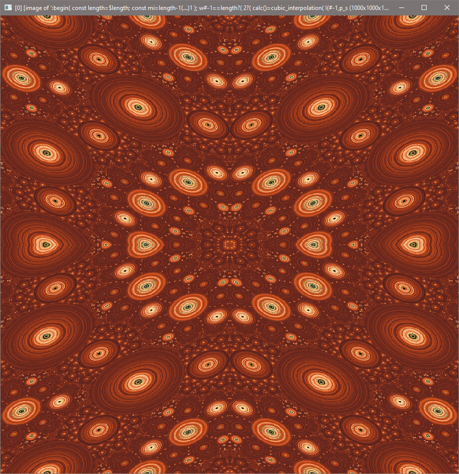
Looks fun.  With some colours, it would be amazing.
Sort of related… back when I used to write some graphics things in assembler, I once had a flawed program start executing data. By chance, it produced the most incredible patterned animation. We could only stare in amazement, knowing that after a reboot it would almost certainly never be reproduced (it wasn’t, and yes I did try!).
Still thematically similar in colour but I understand it is a WIP. 
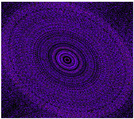
Here it is. I’ll be happy to explain any part of it. Coordinates x and y are converted to indices into a matrix. Every time a matrix element is hit, it is incremented by one. The matrix is displayed as a heatmap.
function run(tries=1000; h = 400, w = 400)
    Z = zeros(Int, h, w)
    for _ in 1:tries
        sercir!(Z)
    end
    imagesc(Z)
end

# values outside the "viewport" are shifted back into it.
function wraparound(x, xm, xM)
    while x < xm
        x += xM-xm
    end
    while x > xM
        x -= xM-xm
    end
    return x
end

function sercir!(Z,
                 # initial value
                 xi   = 6*rand()-3,
                 yi   = 6*rand()-3;
                 # "viewport"
                 xr   = (-2.0, 2.0),
                 yr   = (-2.0, 2.0),
                 reps = 10000)

    h, w = size(Z)
    x, y = xi, yi
    xm, xM = xr[1], xr[2]
    ym, yM = yr[1], yr[2]

    for _ = 1:reps
        x = x - y/2
        y = y + x/2

        xi = wraparound(x, xm, xM)
        yi = wraparound(y, ym, yM)

        # map `x, y` coordinates to a matrix location
        col = (xi-xm)/(xM-xm)*(w-1)+1
        row = (yi-ym)/(yM-ym)*(h-1)+1

        c = round(Int, col)
        r = round(Int, row)

        Z[r, c] += 1
    end
end
I can’t reproduce Reptorian’s plots with this code, though – all ellipses I get are centered in the origin; only their size changes.
Can you show us the output? I can’t run it.
EDIT:
The only problem I now have is revealing outside of the boundary, and I have to say, that is probably impossible. I only have hints of that.
What do you mean by “reveal outside the border”?
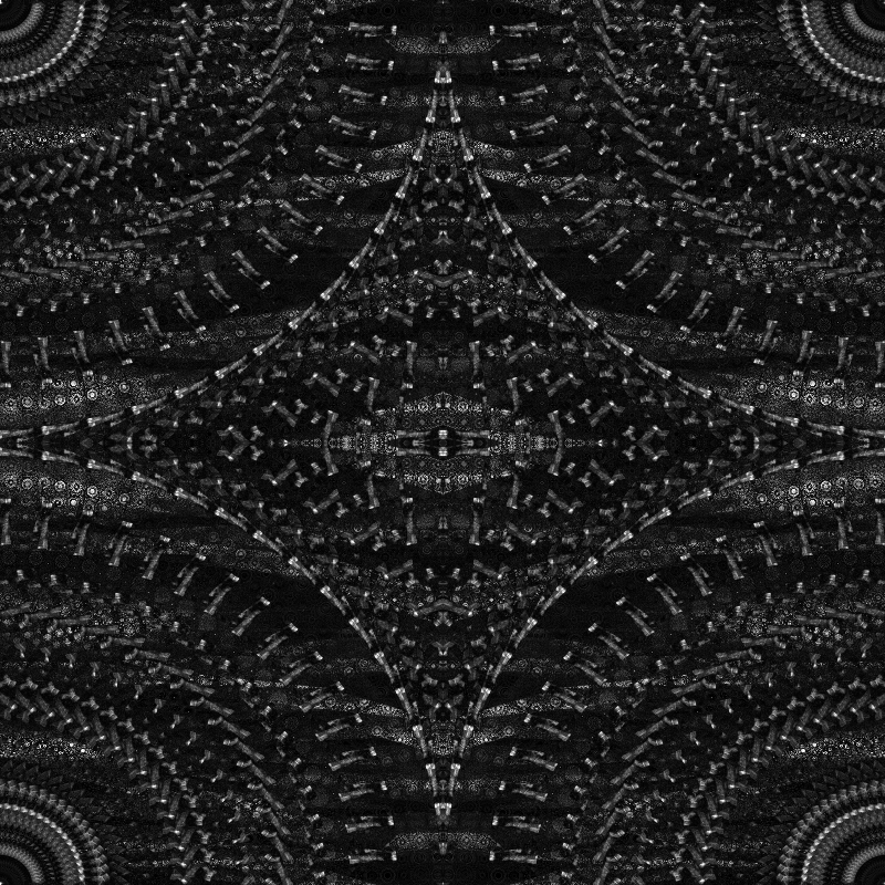
Here’s one example, with random initial values between -3 and 3, with viewport between -2 and 2; values outside the viewport are mirrored back. This is 60 ellipses.

See here:
The left and right side are unfilled. It definitely would be nice if there is another expression that generates similar image, but being able to fill outside of border. But, I won’t look at finding how as basic search for solution haven’t been found, and mathematically, it’s not possible (probably).
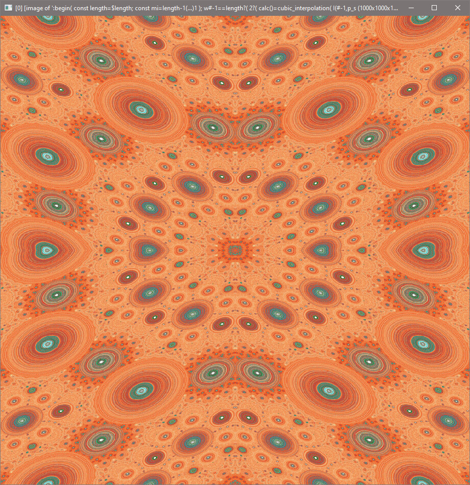
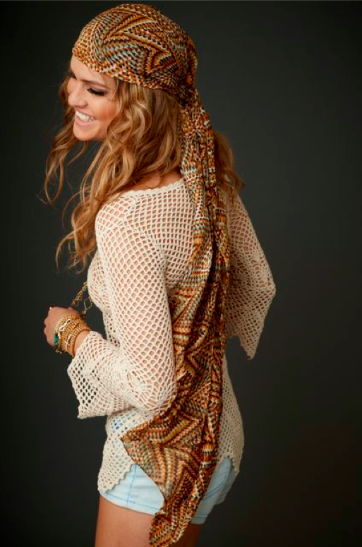
This could be a nice design for some bohemian hippie headscarf 
I finalized the CLI version. Just wish there was percentile-based cut though. Here’s a mixture of 3 Serendiptous Circle.
I recall a command named percentile and another that addresses percentile cuts, but maybe not what you are asking… I am not sure what you are asking…
Basically, what I’m looking for a command that cuts based on the frequency vs dimension ratio. $1 would be the parameter to find the lowest value that has a frequency higher than $1, and $2 would be the parameter to find the highest value that has a frequency higher than $2. Then, cut based on the found values. That’s something I requested on G’MIC 3.1 thread.
Like a band pass/stop? There is a bandpass command that you could use as a starting point.
bandpass:
    _min_freq[%],_max_freq[%]

  Apply bandpass filter to selected images.

  Default values: 'min_freq=0' and 'max_freq=20%'.

  Example:
    [#1] image.jpg bandpass 1%,3%

  Tutorial: https://gmic.eu/oldtutorial/_bandpass
That doesn’t give me the output I want. I want to cut instead. Let me see. I could try to do a custom command involving sorting, and then find the frequency of each value, and cut based on those.
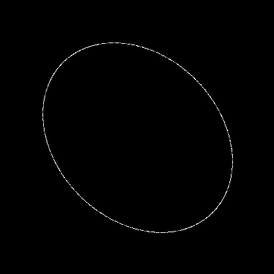
The world doesn’t have enough graphics languages, so here’s a solution in “alfim”, a language I am developing. I call sercir() only once, so there is only one “circle”. It is based on code above by @mbs, but with smaller initial (xi,yi) and without wraparound.
function sercir ()
  variables
    WW = %[fx:w],
    HH = %[fx:h],
    xi = %[fx: 4 * rand() - 2],
    yi = %[fx: 4 * rand() - 2],
    xmin = -2,
    xmax = +2,
    ymin = -2,
    ymax = +2,
    xmult = %[fx: (%{WW}-1) / (%{xmax}-(%{xmin})) ],
    ymult = %[fx: (%{HH}-1) / (%{ymax}-(%{ymin})) ],
    rep = 1,
    col,
    row,
    x = %[fx: %{xi} ],
    y = %[fx: %{yi} ]
  endvariables

  -fill White

  while %[fx: %{rep} < 1000 ] do

    assign x = %[fx: %{x} - %{y}/2 ]
    assign y = %[fx: %{y} + %{x}/2 ]

    assign col = %[fx: (%{x}-(%{xmin})) * %{xmult} + 1 ]
    assign row = %[fx: (%{y}-(%{ymin})) * %{ymult} + 1 ]

    -draw "point %{col},%{row}"

    assign rep = %[fx: %{rep} + 1]
  endwhile

endfunction

-size 400x400 xc:Black
call sercir ()
+write x.png
Sounds like you’re talking about statistical relative frequency? A histogram ought to manage that…
What I understand here is what you name “frequency” is actually the “occurence”, right ?
(Frequency in image often refers to Fourier decomposition in image processing).