So, here are the math tricks I used to find a parameterization of the “rectangle spiral”.
I’ve decomposed the problem into two sub-problems:
1. Find a parameterization of an outlined rectangle of size w x h:
What we want here is a parameterization such that when t increases, the set of points (x_t,y_t) draws a rectangle of size w\times h. More precisely, we want it to draw first the segment (0,0)\rightarrow(w-1,0), then the segment (w-1,1)\rightarrow(w-1,h-1), then (w-2,h-1)\rightarrow(0,h-1) and finally (0,h-2)\rightarrow(0,1).
Note that the number of pixels that compose the outline (the perimeter) is given by:
P(w,h) = (w) + (h-1) + (w-1) + (h-2) = 2\;(w + h -2)
which means that the parameter t has to go from 0 to P(w,h)-1 (included).
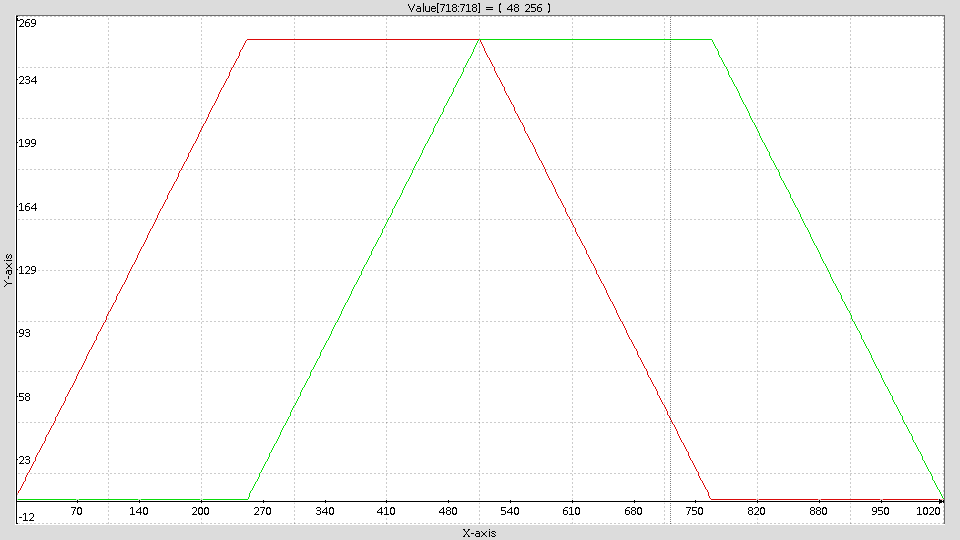
For instance, for a 256\times 256 image, we’ll get P(256,256) = 1020 pixels composing the rectangle outline.
Here is the expected graph of the x(t) (in red) and y(t) (in green) coordinates, for t going from 0 to 1019:
Each curve is composed of linear parts (with a slope of
1 and
-1), as well as constant parts whose values are
0 and
255.
Actually, looking at these curves, we can easily get the feeling that they can be modeled by saturated, shifted and inverted absolute values of
t, i.e.
x_t = a_x - | t - b_x |~~~~\text{and}~~~~ y_t = a_y - | t - b_y |
where a_x,b_x,a_y and b_y are constants to be determined, which is somehow easy, as we expect that:
x_0 = 0~~~~\text{and}~~~~x_{(w+h-2)} = w-1
which gives a_x = b_x = \frac{2w + h - 3}{2} . Same for y_t, with the conditions
y_{(w-1)}=0~~~~\text{and}~~~~y_{(2w+2h-4)}=0
which gives b_y = \frac{3w + 2h - 5}{2} and a_y = b_y - w + 1.
Adding the value cut in the ranges [0,w-1] (for x_t) and [0,h-1] (for y_t) does the trick.
Here is the curve obtained with x_t = a_x - | t - b_x | (in red), and its saturated version (in green), which is exactly what we are looking for.
So, at this point, we have a parameterization of the very first part of the “rectangular spiral”, which is the outline of the rectangle with size w\times h (shown below for a 16\times 16 image):

The complete spiral is in fact composed of several outlines like this, where the origin of the drawing starts from (0,0), then (1,1), (2,2), etc… and where the dimensions of the drawn rectangle outlines decreases : (w,h), (w-2,h-2), (w-4,h-4), etc…
So now, we have to “link” all these rectangle outlines together in a single parameterized function, and this is the goal of the second part.
Link all rectangle outlines together
Of course, we could have just made a loop, let say from \alpha = 0\dots\alpha_{max} (\alpha being an integer) and draw each rectangle outline starting from point (\alpha,\alpha) with size (w - 2\;\alpha,h - 2\;\alpha), but this wouldn’t be funny. We want a single parameter t for the rectangular spiral, (so a single loop), not two distinct parameters (nested loops)!
So now, the problem is to find for each t from 0 to w\times h-1 (which is enough to scan all the pixels of a w\times h image), in which rectangle outline (i.e. which value of \alpha) we are located, as well as the relative position of the point (x_t,y_t) in this outline. What makes this complicated is that the perimeter P(w,h) of each rectangle is decreasing each time a new rectangle is drawn (because each time, the width and height of the rectangle lost 2 units), so there is not a constant period we can rely on to easily find \alpha. See \alpha as the level of interiority of the rectangle outline we are drawing for a certain value of the parameter t. \alpha is of course a function of t, so let us denote it by \alpha_t.
This is obviously an increasing function that starts from \alpha_{(0)} = 0.
How to determine \alpha_t from t ?
We denote by \mathcal{P}(\alpha_t) the sum of the perimeters of the \alpha rectangle outlines when they are completely drawn. It’s easy to see that
\mathcal{P}(\alpha_t) = \sum_{k=0}^{\alpha_t-1} P(w-2k,h-2k) = \sum_{k=0}^{\alpha_t-1} 2w + 2h - 4 - 8k
= \alpha_t\;(2w + 2h - 4) - 4(\alpha_t-1)\alpha_t
= -4\;\alpha_t^2 + 2\alpha_t\;(w + h)
And the thing is that our desired parameter t has been designed exactly to count the number of pixels that have been drawn. So, for each t corresponding to the end of an outline drawing, we’ll have t = \mathcal{P}(\alpha_t). As \mathcal{P}(\alpha_t) is an increasing function, we can determine \alpha_t by taking the floor() of the solution to the equation
t = \mathcal{P}(\alpha_t)
which means we just have to solve this second-order polynomial:
4\;\alpha_t^2 - 2\alpha_t\;(w + h) + t = 0
That is trivial, and the interesting (rounded to lower integer) solution we get is:
\alpha_t = \text{floor}\left(\frac{1}{4}\;\left((w + h) - \sqrt{(w+h)^2-4t}\right)\right)
We are almost done. For any t from 0 to w\times h-1, we can now determine the level of interiority \alpha_t of the drawn outline.
The graph below shows the evolution of \alpha_t for a 64\times 64 image (t being on the horizontal axis). We can see that, as expected, \alpha_t is an increasing integer, and it increases faster as t goes on.
Now that we know in which rectangle outline we are, we just have to find the relative position of the outline drawing from its starting position t_0, which is easy to compute as t_0 = \mathcal{P}(\alpha_t).
Then, we know everything to plug the different outline drawing functions together : the starting parameter t0, the level of interiority \alpha_t, the width and height of the rectangles w-2\alpha_t and h-2\alpha_t, as well as the starting pixel (\alpha_t,\alpha_t).
Summary
At the end, the (x_t,y_t) coordinates that describe the “rectangular spiral” for an image w\times h are given by:
\left\{
\begin{array}{lcl}
x_t & = & \alpha_t + \max(0,\min(w_t-1,a_t^x - |t - t0_t - a_t^x|)) \\
y_t & = & \alpha_t + \max(0,\min(h_t-1,a_t^y - | t - t0 _t- b_t^y |))
\end{array}
\right.
with
\alpha_t = \text{floor}\left(\frac{1}{4}\;\left((w + h) - \sqrt{(w+h)^2-4t}\right)\right),
t0 = 2\alpha_t(w + h) - 4\alpha_t^2,
w_t = w - 2\;\alpha_t, ~~~~h_t = h - 2\;\alpha_t,
a_t^x = \frac{1}{2}(2w_t + h_t - 3), ~~~~b_t^y = \frac{1}{2}(3w_t + 2h_t - 5),~~~~a_t^y = b_t^y - w_t + 1
Below is the graph of the x_t (in red) and y_t (in green) obtained with this parameterization, for a 32\times 32 spiral image:
And the resulting 2D image is

Job done 
Note that in practice, implementing this parameterization is not particularly interesting for drawing the “rectangular spiral”, as it involves more operations that doing it with nested loops or using multiple variables (just as @garagecoder did in its version).
Inverting parameterization for parallel implementation
I have been wondering this morning, if this parameterization could be inverted, i.e, if we are able to easily retrieve t given x_t,y_t. That would mean the computation of t could be done in parallel.
It turned out that it was easier than expected
First, we notice that the degree of interiority \alpha_t of a rectangle can be evaluated for a pixel x,y of the image as
\alpha_t = min(x,y,w-1-x,h-1-y)
Thus, we can compute t0 = P(\alpha_t) = 2\alpha_t(w + h) - 4\alpha_t^2, the t that corresponds to the start of the interior rectangle outline on which the pixel (x,y) is located.
The dimensions of this rectangle are given by W = w -2\alpha and H = h - 2\alpha.
To evaluate the relative parameterization of (x,y) inside this outline, we determine in which segment of the rectangle outline the point (x,y) is located, and we then deduce t - t_0 to be
t - t_0 = \left\{
\begin{array}{ll}
x - \alpha_t,&~~~\text{if}~y - \alpha_t = 0\\
W - 1 + y - \alpha_t,&~~~\text{if}~x - \alpha_t = W-1\\
2W+H-3 - x + \alpha_t,&~~~\text{if}~y - \alpha_t = H-1\\
2W+2H-4-y + \alpha_t &~~~\text{otherwise}
\end{array}
\right.
This means it is possible now to write a parallel implementation of command spiralbw, that looks like this:
spiralbw_parallel :
  $1,$2,1,1,"
    alpha = min(x,y,w-1-x,h-1-y);
    t0 = alpha*2*(w+h) - 4*alpha^2;
    X = x - alpha;
    Y = y - alpha;
    W = w - 2*alpha;
    H = h - 2*alpha;
    t = t0 + (Y==0?X:
              X==W - 1?W - 1 + Y:
              Y==H-1?2*W+H-3 - X:
              2*W+2*H-4 - Y)"
Looks great isn’t it ?  I didn’t compare the timings yet, but for large images it should be really interesting. I’ll probably update the command
 spiralbw in the G’MIC stdlib.
I think I’ve finished with the math of the “rectangular spiral” now !


 It is much clearer to me now, though I still need to go through it step by step.