Just noticed that you added collages to all sets of ‘Color Preset’ and ‘Film Simulation’.
Thanks for that, it does make it easier to discover inspiring CLUTs for a picture.
1 Like
Is there a link to access this 2.5Mb file ?
This file: Sign in · GitLab
EDIT : A PNG version of this file is available here : Sign in · GitLab
(basically, one row = one clut).
1 Like
congrats on the paper, this is a nice read. you didn’t end up to do the comparison to radial basis function interpolation in this write up? do you still have any numbers on that? i’d be interested what my trade off options are here  like what is the tipping point when the RBF become more expensive or what is their accuracy at same memory usage.
2 Likes
That is unfortunately not possible to do this in a reasonable time using the algorithm we propose to add keypoints. Once the number of keypoints becomes higher than, let say, 200, the reconstruction time of the entire CLUT volume becomes really slow.
And most of the time, we need more than 200 keypoints.
I’ve tested with some “simple” CLUTs that requires only a few keypoints, and I didn’t notice that the RBF reconstruction produces less keypoints in general (sometimes, it does, sometimes not, depending on the CLUT content).
1 Like
Some news:
I’ve discovered FreshLUTs yesterday, and decided it was time to add a few more CLUTs to G’MIC ! So I’ve downloaded some of CLUTs from this website, and compressed them.
Right now, we have then 716 compressed CLUTs available in G’MIC (stored in a single 3Mb file).
I’ve updated the data files on my libclut repository.
And I’ve also added the new CLUTs directly in the filter Colors / Color Presets available in the G’MIC-Qt plug-in.
3 Likes
Update:
I’ve worked hard these last days, trying to improve my CLUT compression algorithm even more. I found a slight improvement, by mixing RBF and PDE reconstruction.
I guess this could interest @hanatos. So I briefly explain the idea here:
Observations:
Basically, what I’ve noticed is that some CLUTs are really well compressed with the RBF reconstruction method (Radial Basis Function), and not so well with the PDE-based method.
But It really doesn’t happen very often. It’s only for a few CLUTS (like <10% or the set of 715 CLUTs I have), that probably have an internal structure where splines can fit the data particularly well
(so, usually, very smooth CLUTs without discontinuities, etc.). Typically CLUTs that looks alike the identity CLUT.
Proposed solution:
So for these CLUTs, the RBF is better, and as in this case, the number of needed keypoints is quite low (generally less than 200), it was a bit a shame to not using RBF for these particular CLUTs.
My proposal, which seems to work reasonably well, is to mix the RBF and the PDE reconstruction of the CLUT, in order to reconstruct a CLUT from its set of colored keypoints, and use this mixed reconstruction method in the compression algorithm I’ve proposed in the paper we wrote (see first post). I’ve tried different ways of mixing the two approaches, and what worked the best is simply a linear mixing:
\text{CLUT}_{mixed} = \alpha\;\text{CLUT}_{RBF} + (1-\alpha)\;\text{CLUT}_{PDE}
\text{where}~\alpha~\text{is the current number of keypoints that represents the CLUT, defined as:}
\alpha = \max(0,\frac{320-N}{320-8})
so it goes from 1 (where N=8, i.e. at the CLUT initialization, to 0 , where N>=320, which is the limit I’ve set. When this limit is reached, the RBF reconstruction is disabled (it takes a lot of time, when the number of keypoints become high).
Results:
I’ve re-run the compression algorithm for the CLUTs that were using less than 1000 keypoints, and there is a small improvement in the size of the compressed data.
We go from 3115349 bytes to 3019013 bytes, so about 96Kb of saving. That’s not really spectacular, but at least I’ve tried something new
All the experiments I’ve made made me realize that on average, there are not much differences in quality between the RBF and PDE reconstruction. Sometimes the former compresses some CLUTS better, sometimes it’s the latter. That really depends on the CLUT structure. The big difference that counts is on the reconstruction time, where the RBF becomes painfully slow when the number of keypoints increases significantly.
That’s all for tonight
5 Likes
Update: (probably the last about this topic!).
I’ve made a few other experiments, and finally noticed that in general it’s more efficient not to linearly mix the RBF/PDE approach for CLUT compression.
What is clear to me now is that when the RBF approach works well for one CLUT, it works better alone (not with a PDE counterpart). This is basically due to the fact that the CLUT has been probably designed from tools that are themselves spline-based, so the RBF approach fits the data very well.
For other kind of CLUTs, the PDE approach is more efficient (in terms of computation speed, while keeping the same compression ability).
So what I’ve done is : for all CLUTs that could be compressed efficiently with the RBF approach alone with a small amount of keypoints (which means <320 keypoints, this concerns 255 / 716 CLUTs), I’ve kept the RBF approach. All other are compressed with the PDE approach. Thus, I get a good balance between good compression size and efficient time for the decompression.
This is what is now implemented in G’MIC. This way, I’ve been able to store the 716 CLUTs in a file having a size of 2706237 bytes (2.7Mio), this saves again 300Kb from my previous attempt.
I’ll probably stop my experiments here. I’ve tried literally dozens of compression/decompression variants, tweaking the parameters like crazy, and I’m not sure saving another tens of Kb is worth it.
After all, I’ve already reached a compression rate of 97%+, if we compare the CLUT size with the original data in .png and .cube format (which were already compressed!).
Not so bad 
2 Likes
great, thanks for the update. so you’re saying 320 points is the turnaround point for precision? or for your pain threshold with respect to speed of the implementation? i’m still interested in your perf numbers here.
Yes, that only concerns the speed of the implementation.
My RBF decompression is written as a G’MIC script here, so not that fast (but parallelized anyway).
I’m pretty sure a C++ version of the RBF decompression would perform better, but at the same time, I didn’t noticed that for a high number of points (i.e. >300), the RBF approach performs particularly better than the PDE technique.
It works really well in some cases, because of the nature of the CLUT to compress (probably the ones that have been generated following a spline or a linear model). For more complex CLUTs, both RBF/PDE approach give roughly equivalent results (in number of keypoints).
Some numbers, to get an idea.
I’ve 716 CLUTs compressed for now.
Here is the number of keypoints (y-axis) for each CLUT (x-axis), sorted by increasing number of keypoints.
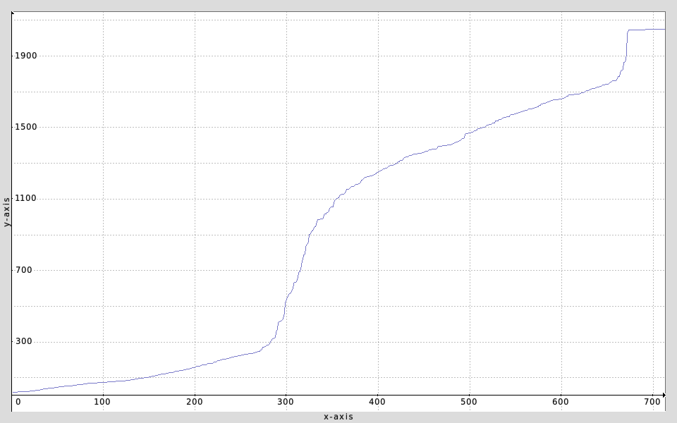
There is a visible limit, at around y = nb_keypoints = 280, where the number of required keypoints for compressing a CLUT becomes high ‘by nature’ (that’s why I chose the threshold to be 320). This is actually independent to the decompression method chosen (RBF/PDE). It says that CLUTs which needs usually more than 280 keypoints to be compressed often requires a lot of keypoints (most requires 1000+). There are very few CLUTs that are efficiently compressed with a number of keypoints between [280,1000].
Here is the histogram of the number of keypoints for the 716 CLUTs.
I’ve used 32 bins, from 0 keypoints to 2047, which means each bin k corresponds to the number of CLUTs that require between 64*k and 64*(k+1) keypoints to be compressed:

As you can see, there are clearly two modes : the “easy CLUTs” (left part), and the “hard CLUTs” (right part), and very few CLUTs exists between these two worlds.
Here are some decompression timing, on a i7 with one or several cores, for a 64^3 CLUT decompression (using 320 keypoints, comparing PDE/RBF decompression)
$ OMP_NUM_THREADS=1 gmic gmic_cluts.gmz k[paladin] rows 0,319 tic decompress_clut_pde 64 toc
→ Single core : PDE=4.65 s, RBF=23.951 s
$ OMP_NUM_THREADS=4 gmic gmic_cluts.gmz k[paladin] rows 0,319 tic decompress_clut_pde 64 toc
→ 4 cores : PDE=1.572 s, RBF=6.761 s
$ OMP_NUM_THREADS=32 gmic gmic_cluts.gmz k[paladin] rows 0,319 tic decompress_clut_pde 64 toc
→ 24 cores : PDE=0.635 s, RBF=1.843 s
(The RBF approach is more easy to parallelize than the PDE one, hence the reduced difference when the number of cores becomes higher).
Both methods are written as G’MIC scripts, so they are comparable in term of timing. It is actually coherent with the theoretical algorithmic complexity they have.
1 Like
nice! these numbers are super interesting, thanks for sharing! now it seems clear where your threshold of 320 comes from. interesting to see how it’s separated into the two modes. i wonder into which class lut profiles would fall, which map camera rgb to true xyz values. and yes, you would expect the RBF to have terrible scaling with the number of points.
1 Like
A small update:
The article we have written about the CLUT compression method used in G’MIC, has been accepted for publication at the CAIP’2019 conference (18th International Conference on Computer Analysis of Images and Patterns). That is great news!
We are currently writing a long version of the paper for a submission to a journal (which one is not decided yet).

We have also a French version of the paper, that has been accepted at the GRETSI’2019 conference (the main French conference about image and signal processing). which will be held in Lille / France, at the end of August.
Reviews for both English/French versions of the paper were really great, with no major concerns from the reviewers. That’s always nice to know we don’t have a lot of work to do before submitting the final version
Now, we have to prepare the slides and/or posters for the presentations.
Still a lot of work to do, but having our work published somewhere as a scientific paper and at the same time implemented in an image processing software so that users around the globe can benefit from it is really satisfying for us (but it also doubles the amount of work, compared to a more classical research-only paper ).
10 Likes
The slides for the conferences are now ready!
Next two weeks, we have first a presentation at the GRETSI’2019 conference in Lille / France, then to the CAIP’2019 conference in Salerno. A busy start to the school year! 
3 Likes
A small update :
We have finally a long version of this CLUT compression work that has been accepted and published in SIIMS (SIAM Journal on Imaging Sciences), a good journal in our community.
We have also a reformatted version available on HAL (French equivalent of Arxiv), with lot more details and stuffs than in the CAIP’2019 conference paper.
You can get the .pdf here : https://hal-normandie-univ.archives-ouvertes.fr/hal-02940557/document
Probably not of broad interest, but maybe @hanatos could be interested ? (a bit of RBF inside ).
2 Likes
nice, thanks for the pointer. this has become quite an extensive writeup! i like the new visualisations of the RBF
i’m using what @gwgill called 2.5D luts in vkdt now for colour mapping. that is, a 2D thin plate spline RBF (i.e. log something radial function) on xy chromaticity values (or some similar space based on unbounded rec2020 rgb values), normalising away the input brightness (X+Y+Z, proportional to radiance or so). that’s because i’m mostly interested in replacing the dreadfully wrong input colour matrix transform by something better.
i’m hoping to do gamut mapping by just moving the control node points inwards, but didn’t push this to production quality yet.
1 Like
Did a talk today about CLUT compression/decompression in G’MIC. Just in case ![]()
.")
1 Like
really liked it, especially the practical part
Saw 5 or 10 minutes of the beginning (friends came around). Quite technical I thought…
Perhaps, in time, libraries of CLUTs will disappear. For I start with a good quality image that — for all its quality, does not convey the mood of my contemplated production. So after much work, some consultation, a bit of staring moodily out of windows, entertaining one or two thoughts that — in the next life — I shall take up something simple, possibly brain surgery, I arrive at an adjusted image that conveys the mood. Implicit between those two images is a CLUT. And that CLUT is not so much of a Holy Grail, just working data. The Holy Grail is, instead, that pair of images. And I might tweak one or another to generate a family of CLUTs, to be used and then cleared from storage when I need some space. But those two images — Ha! — They go in the vault.