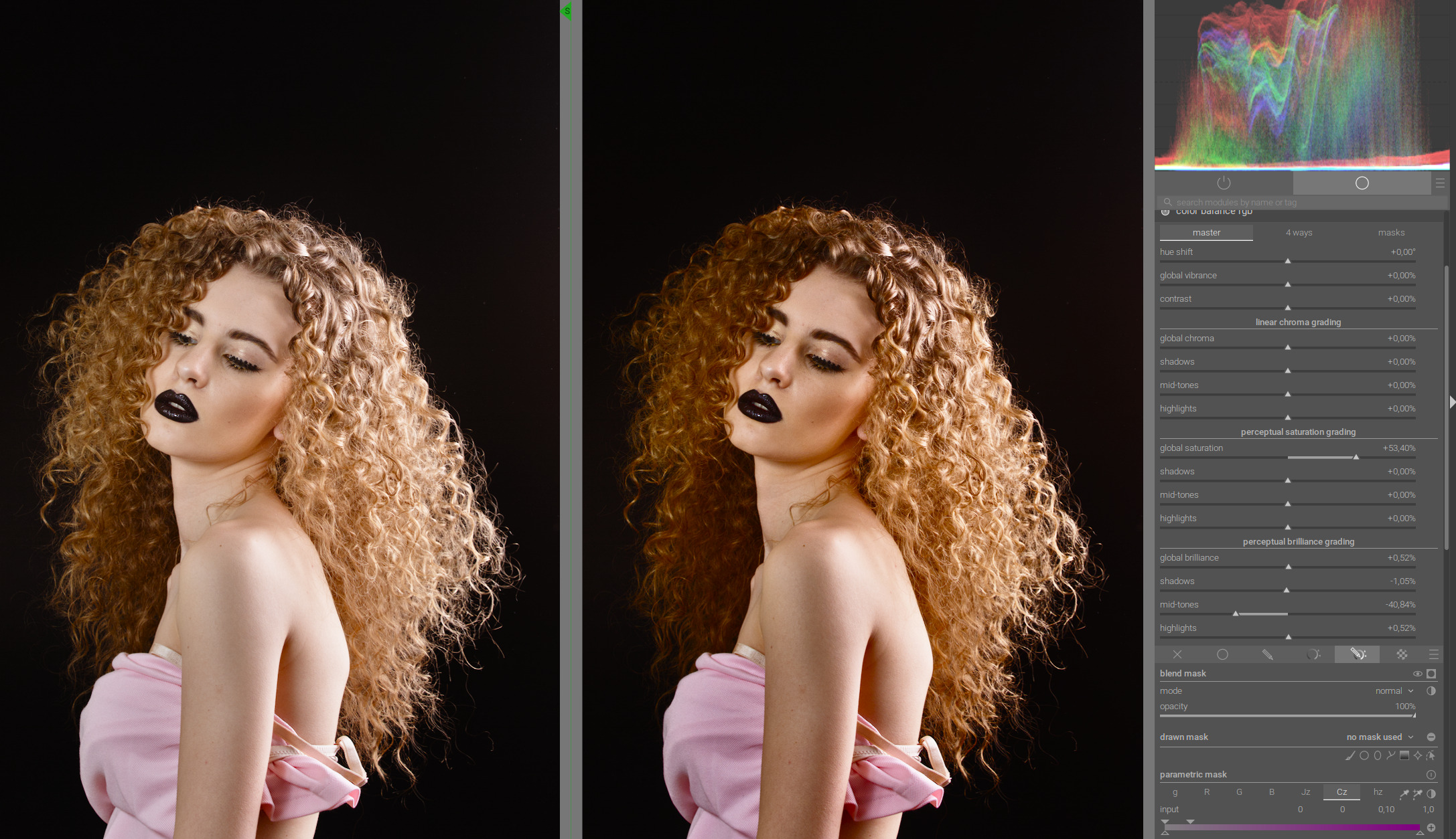
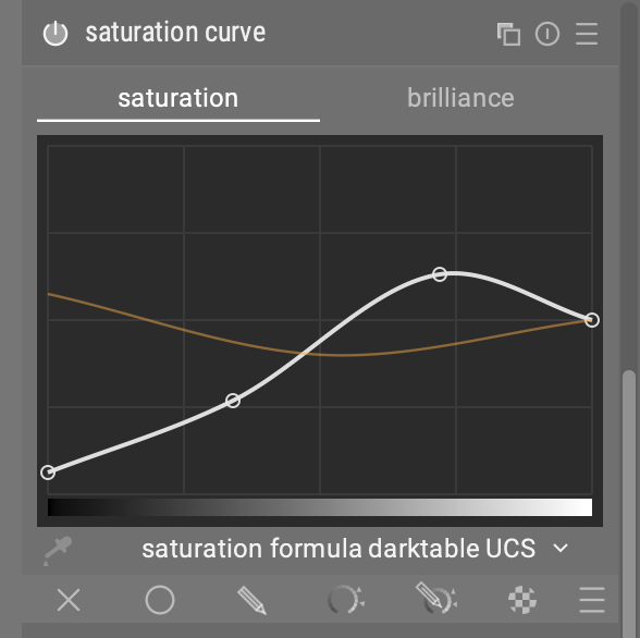
since i frequently used the sat vs sat curve in davinci resolve i played around with a couple of agents to help me get such thing for darktable:
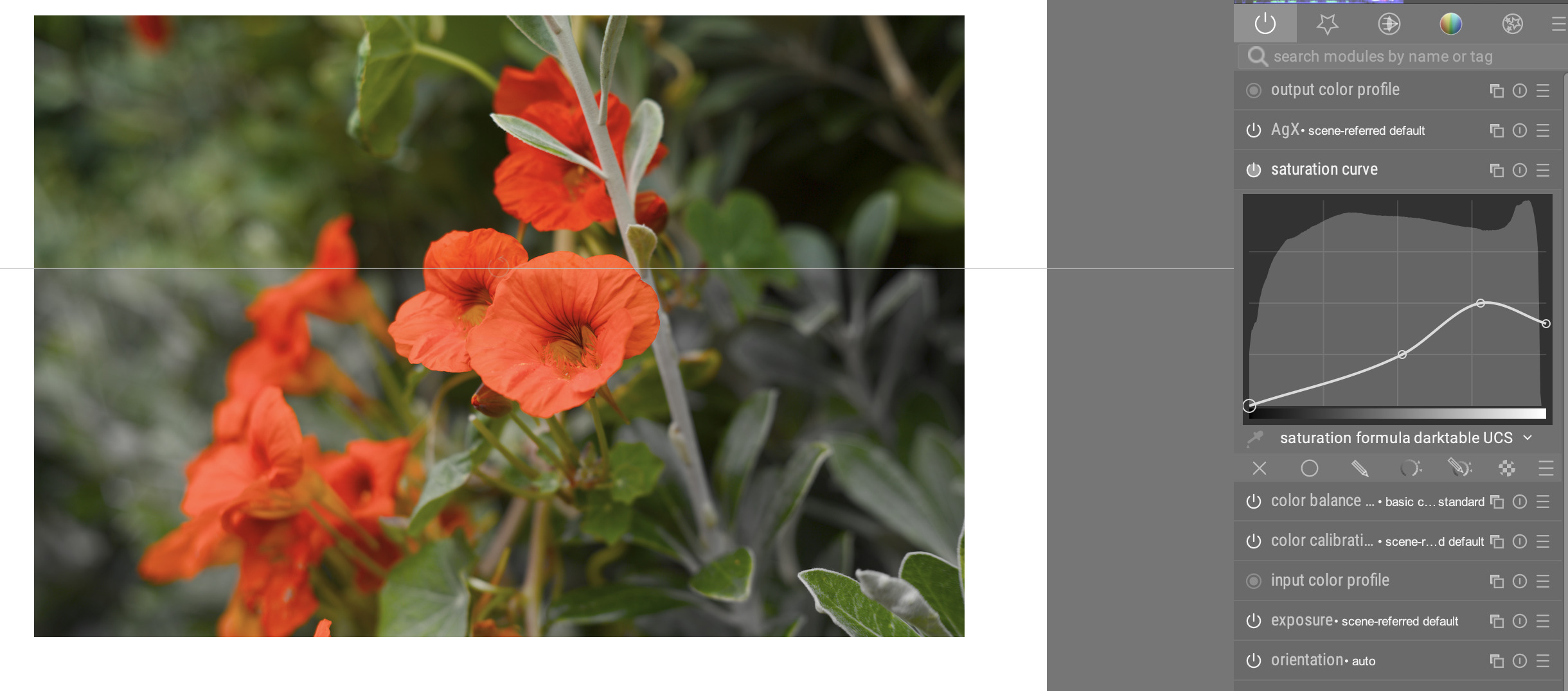
No rocket science, just an adaption of the perceptual saturation handling of colorbalance rgb but based on input saturation. So this can be done also with colorbalancergb and parametric masking (maybe more than one instance)
quite simple UI:
- curve area left → right: lowest to higest saturation
- curve upwards increases saturation, downwards decreases
- click on curve to create a node, right click to remove
- color picker to show the saturation
- two saturation modes: JzAzBz and darktable UCS
if interested in playing around with it: https://github.com/MStraeten/darktable/tree/satcurvergb
Claude generated Documentation
description : remap saturation with a curve
purpose : corrective or creative
input : linear, RGB, scene-referred
processing : linear, RGB, scene-referred
output : linear, RGB, scene-referred
saturation curve remaps an image’s saturation through a freely editable curve, plotted against the input saturation itself. Unlike a global saturation slider, it lets you raise or lower different saturation ranges (muted vs. already-vivid colors) independently.
Aliases: sat vs sat, saturation versus saturation, satcurve.
introduction
A global saturation slider scales all colors equally, regardless of how saturated they already are. This often pushes already-vivid colors into gamut clipping first, while muted colors barely benefit. saturation curve addresses this by using the input saturation itself as the curve’s x-axis: y-values above 0.5 boost saturation in that input range, y-values below 0.5 reduce it, and y = 0.5 leaves it unchanged. This makes it possible to, for example, lift skin tones (low to mid saturation) selectively without pushing already-punchy colors further – or the reverse.
general principles
The module works in two steps:
- For each pixel, a normalized input saturation
S_in_normis computed (range 0–1, where 1 corresponds to the maximum saturation representable in the working color space for that particular hue). S_in_normis used as the x-value on the curve; the returned y-valuecscales the pixel’s saturation by a factor of2·c.
Why the gamut normalization: without it, “saturation = 1.0” would sit at a different distance from the gamut boundary depending on hue, and the curve would have to be interpreted differently per hue. Normalizing means x = 1 always represents “gamut-maximal saturation” for the pixel’s own hue.
saturation formula
Two saturation definitions are available (combobox below the curve graph):
JzAzBz : S_in = Cz / Jz in JzAzBz. Not perceptually linear with respect to the Helmholtz-Kohlrausch effect.
darktable UCS : Saturation in the darktable UCS color space (HSB representation, S = HCB[1] / HCB[2]). The module’s default. Accounts for the Helmholtz-Kohlrausch effect and behaves more evenly across the lightness range.
Why this is a user choice rather than fixed: S_in_norm is defined differently per formula, so this setting is technically part of the curve itself rather than a separate tab. Switching the formula invalidates the histogram and, in effect, any curve points already set, since the meaning of the x-axis changes.
For the gamut reference, both formulas use a hue-indexed gamut LUT (92³ RGB samples for JzAzBz, a dedicated routine for darktable UCS), which is rebuilt whenever the working profile changes.
anti-clipping
The output value is not hard-clipped at the gamut boundary; from 80% of the maximum representable saturation onward it asymptotically approaches that boundary (a soft knee). For the JzAzBz formula, the module additionally checks that the JzAzBz → XYZ back-transform does not produce negative L’M’S’ values; if it would, chroma is clipped further.
Why: a hard clip would create visible contouring near the gamut boundary under strong curve boosts. The soft transition avoids this at the cost of slightly reduced effect near the limit.
module controls
curve graph
The x-axis shows S_in_norm (0–1), the y-axis the curve value (0–1, neutral at 0.5). Up to 20 control points, interpolated with a monotone Hermite spline (prevents overshoot/undershoot between points).
- Left-click on empty area: insert a new node
- Drag: move a node (endpoints are locked to x = 0 and x = 1)
- Right-click on a node: remove it (or, with only 2 nodes present, or with Ctrl held: reset it to y = 0.5)
- Double-click: reset the entire curve to its neutral state
A histogram of S_in_norm across the current image is drawn in the background (log1p-scaled, since the distribution is usually heavily skewed toward low values). Below the graph sits a purely decorative hue gradient bar for orientation.
color picker
The picker button next to the formula combobox computes S_in_norm for the picked region and overlays them on the graph as a vertical line. This shows directly where a given subject falls on the curve’s x-axis before you place a node there.
presets
neutral : 2 nodes, curve = 0.5 throughout, no effect.
gentle saturation : 2 nodes, y slightly above 0.5 across the full range – a flat, global saturation lift.
protect saturated colors : 3 nodes, mid saturation lifted, high saturation lowered – protects already-vivid colors from further clipping.
boost saturated colors : 3 nodes, low saturation lowered, high saturation lifted – the inverse of protect saturated colors.
internal processing
Per-pixel flow (simplified, for darktable UCS):
- Pipeline RGB → XYZ (D50→D65, working profile matrix)
- XYZ → xyY → dt UCS JCH → HCB → HSB
S_in_normfromHSB[1] / HSB[2], normalized against the hue-dependent gamut boundary- Curve LUT lookup returns
c;HSB[1] *= 2·c - Soft clip of
HSB[1]against the gamut boundary - HSB → JCH → xyY → XYZ → pipeline RGB
For JzAzBz the flow is analogous, but operates on Jz/Cz/h instead of JCH/HSB.