G’MIC Adventures #5: Multi-Layer Perceptron Tries to Reproduce an Image

[David_Tschumperle (G'MIC staff)]

Hi everyone,

I was itching to do another episode of gmic-adventures, so here it is, and this time we’re going to (finally!) start talking about (small) neural networks!

Introduction

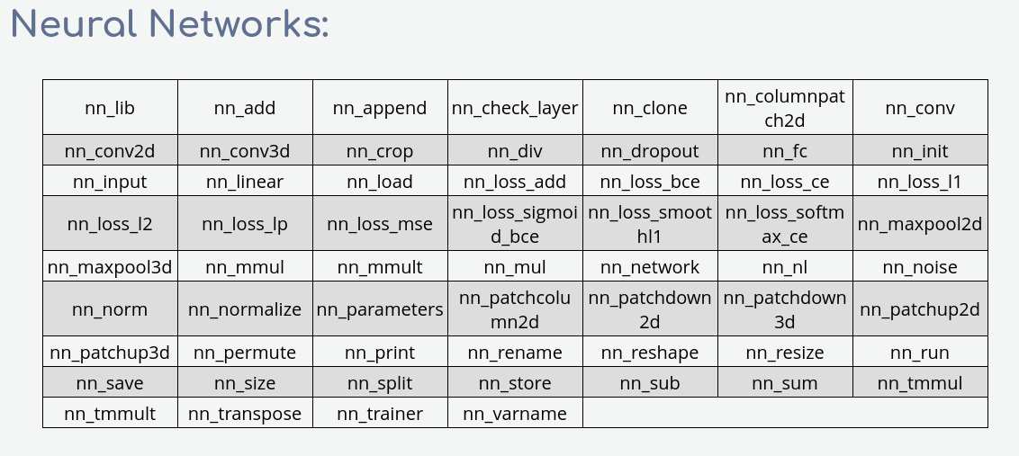
As you know, I have been trying for a few years now to develop a small library (called nn_lib, for “neural-network library”) in order to manage neural networks directly within G’MIC, and I think it’s time to illustrate its use with a simple example.

And what are the simplest neural networks imaginable? MLPs (Multi-Layer Perceptrons), of course! If you are unfamiliar with the concept of MLPs, I suggest you consult the Wikipedia page, which will provide much more information than I could give you here.

But basically, an MLP can be seen as a complex mathematical function that takes a vector IN\in\mathbb{R}^m of any dimension m as input, and outputs also a vector OUT\in\mathbb{R}^n (which may have a different dimension n\neq m).

This MLP function has a certain structure that is basically a sequence of matrix products, additions and non linear functions (activations), all these operations being entirely defined by many parameters (usually several thousand or even millions, for instance used to define the matrix coefficients when doing matrix multiplications). The good thing is that you don’t have to find the parameters by yourself, they will gradually be learned during the training phase of the MLP network, in order to estimate an OUT vector that suits us when we give it a given IN vector as input. And that’s precisely the role of the nn_lib :

• Provide a mechanism and a corresponding API to allow neural network training, such that the network weights are learned iteratively from sets of known (IN,OUT) pairs (which constitutes the so-called training set).
• Once the network is trained, nn_lib allows the user to infer the network : he provides an input IN vector, and the library computes the (expected) network output vector OUT.

Depending on the complexity of the considered network, the required size of the training set can be very large, meaning the training can take age (I mean millions of iterations). But for our episode here, I will limit myself to a quite simple MLP network, so the training time will remain acceptable, even with the nn_lib (that only takes advantage of CPU cores).

Objectives

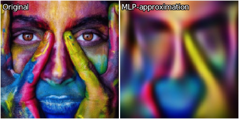
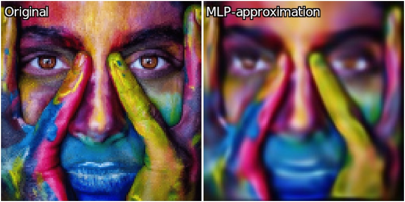
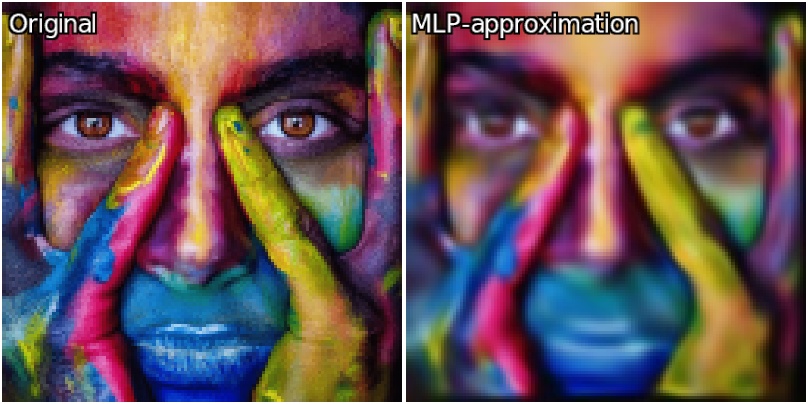
In this episode, my goal is then to show you how to use the nn_lib to quickly design and train a small MLP that takes an input IN\in\mathbb{R}^2 (that represents a coordinate vector (X,Y) ), and estimate an output OUT\in\mathbb{R}^3 (that represents a (R,G,B) color). Thus, we’ll design a network that is intended to learn a complex multi-valued function (X,Y) \rightarrow (R,G,B), from scratch (so basically, a color image!).
I’ll show you how this can be done as a G’MIC script (less than 50 lines of code), and show you then some variations afterwards, for a quick, fun, little trip into the magic world of neural networks.

Important note: We won’t talk about generative AI here, as the kind of networks involved for generative AI are much much larger and complex than the one illustrated here. Neural network is the (current) basis under all the “AI” trend (how much I dislike this term!). And while the use of general AIs may be open to criticism (for many reasons), understanding how neural network algorithms work is really fun and interesting!

Also it’s winter, so make the most of it—with nn_lib, your CPUs will quickly heat up the room!

Spoiler

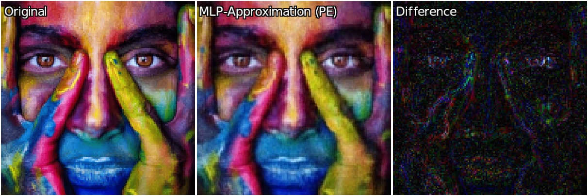
This is a typical result of what our neural network learning algorithm will generate after a few lines of code. In the video below, you can see successive training iterations of a basic MLP, trying to learn one complex function (X,Y) → (R,G,B) (which is here the image produced by the G’MIC command sample colorful).

Stay tuned!

[David_Tschumperle (G'MIC staff)]

How is nn_lib structured?

The nn_lib library is a part of the G’MIC standard library, so it’s already fully integrated into G’MIC. You don’t have to do something special to use it. All functions/commands of the nn_lib have a name that starts with nn_. There is a dedicated section in the G’MIC reference documentation that lists all the corresponding commands (documentation still lacks details though). Here is a screenshot of the list of available nn_lib commands (subject to evolutions in the future of course):

As you can see, the number of functions (60) is relatively small. The whole library takes less than 5k lines of code, in the stdlib. Most of the nn_lib commands are used to define different layer types (or losses) when designing a neural network architecture.

How do I define a MLP with nn_lib?

An example is better than a long speech, so here is how we will define our MLP with G’MIC’s nn_lib:

test_mlp :

  # Define neural network architecture (simple MLP).
  nn_init mlp   # Init new neural network named 'mlp'
  nn_input IN,2 # Input: (X,Y) vector
  repeat 4 { # Define 4 hidden layers (fully-connected layers with sin activations)
    nn_fc FC$>,.,96  # 'nn_fc' adds a 'fully-connected' layer (perceptron) with 96 neurons 
    nn_nl NL$>,.,sin # 'nn_nl' adds a 'non-linearity' layer (here a sinusoidal function).
  }
  nn_fc FC_OUT,.,3 # Last 'fc' layer, return a 3D-vector
  nn_nl OUT,.,sigmoid # Output: the estimated (R,G,B) vector.
  nn_print # Display network information on stdout

The . argument in a function call actually means “previous layer name”, and it’s very convenient to have it, as a neural network is mostly a sequence of pipelined layers/operators.

That’s basically how we tell nn_lib that we want to manage a new neural network mlp.
Let’s test it:

~$ gmic test_mlp
[gmic]./ Start G'MIC interpreter (v.3.7.0).
 * Network name: mlp
   - Layer: IN (type: input)
       * Output: IN (2,1,1,1)
   - Layer: FC0 (type: fc)
       * Input: IN (2,1,1,1) → Output: FC0 (1,1,1,96)
       * Parameters: 288
       * Properties: learning_mode=3, weight_decay=0
   - Layer: NL0 (type: nl)
       * Input: FC0 (1,1,1,96) → Output: NL0 (1,1,1,96)
       * Property: activation=sin
   - Layer: FC1 (type: fc)
       * Input: NL0 (1,1,1,96) → Output: FC1 (1,1,1,96)
       * Parameters: 9312
       * Properties: learning_mode=3, weight_decay=0
   - Layer: NL1 (type: nl)
       * Input: FC1 (1,1,1,96) → Output: NL1 (1,1,1,96)
       * Property: activation=sin
   - Layer: FC2 (type: fc)
       * Input: NL1 (1,1,1,96) → Output: FC2 (1,1,1,96)
       * Parameters: 9312
       * Properties: learning_mode=3, weight_decay=0
   - Layer: NL2 (type: nl)
       * Input: FC2 (1,1,1,96) → Output: NL2 (1,1,1,96)
       * Property: activation=sin
   - Layer: FC3 (type: fc)
       * Input: NL2 (1,1,1,96) → Output: FC3 (1,1,1,96)
       * Parameters: 9312
       * Properties: learning_mode=3, weight_decay=0
   - Layer: NL3 (type: nl)
       * Input: FC3 (1,1,1,96) → Output: NL3 (1,1,1,96)
       * Property: activation=sin
   - Layer: FC_OUT (type: fc)
       * Input: NL3 (1,1,1,96) → Output: FC_OUT (1,1,1,3)
       * Parameters: 291
       * Properties: learning_mode=3, weight_decay=0
   - Layer: OUT (type: nl)
       * Input: FC_OUT (1,1,1,3) → Output: OUT (1,1,1,3)
       * Property: activation=sigmoid

 * Total: 11 layers, 28515 parameters.

As you see, command nn_print is really useful to inspect the network architecture, as it provides a lot of details about the network layers. Here we see that our small MLP has already 28k parameters. We’ll try to make it learn a 128x128x3 image (so 49152 values), so we expect (at least) a bit of compression!

Now, what else do we need to train such a neural network ?

• We first need a so-called “loss function” that will be used to compare the estimated MLP output with a “ground-truth” (the output vector we’d like to get at the end), compute the error between the two and retropropagate this error, so that network parameters can be adjusted to make the network guess something closer to the ground-truth. To add our loss function, we just have to write:

  nn_loss_mse LOSS,.,RGB_TRUTH # Mean-squared loss

where RGB_TRUTH will be the name of the variable we will use to store the ground-truth RGB color.
The mean-squared loss is the most basic kind of losses we can think of. Definitely not the best, but for our example it will be sufficient. There are several kind of loss functions already defined in nn_lib (all commands names nn_loss_* in the array displayed above).

• The last thing missing is a “trainer”, which is the module that will be in charge of updating the network weights, at each training iteration, to make the network converge into something interesting. We define a network trainer like this:

  nn_trainer T,.,adam,2e-4 # Adam optimizer with learning rate 2e-4

(here . refers to the loss function LOSS, as a trainer always takes a loss function as an input).

A trainer basically applies one particular optimizer, and one particular scheduler to train the network. The most popular choice nowadays for the optimizer is the AdamW optimizer (which is the one I chose here), but there are other choices possible in nn_lib. For our purpose, it’s really fine.
Concerning the scheduler (which is: how the learning rate is chosen, during the training iterations), that’s clearly something I need to improve in the nn_lib, right now, there are no really interesting scheduler apart from constant (which is the default).

Once you’ve written that, you’re done defining your neural network. It is ready to be trained. And that is what I will describe in my next post.

Stay tuned!

[David_Tschumperle (G'MIC staff)]

Let’s train the network!

This is where we get into the trickiest part of using nn_lib. Since there are often different variants to train a neural network, and we sometimes want to do very specific operations during the training phase (e.g. data augmentation, tweaking gradients, visualizing inputs/outputs of some modules, etc.), the solution chosen for training a network in nn_lib is slightly more complicated than just having an nn_train command that would do everything magically.

The key point to remember is that the network’s training iteration loop must be written explicitly “by hand,” and that all operations performed by the network’s layers are done within the G’MIC’s mathematical expression evaluator (which already gives an obvious advantage: parallel computing is easy to set up, and that’s where your CPUs can start to heat up ).

But before doing the training iterations, let me just define the (X,Y) \rightarrow (R,G,B) function that I’ll use as the training data:

  # Define (X,Y) -> (R,G,B) function to learn (sample color image).
  sp colorful,128 => img

Now the idea is to iteratively pick a set of random points of the image [img] and use those points as the training batch for each training iteration.

Here is the portion of the code that consitutes the training loop:

  # Train network.
  repeat inf {
    iter=$>

    # Do one iteration of training, with batch size 128.
    128,1,1,1,:${-nn_lib}"           # ':' forces the expression to be evaluated in parallel
      XY = [ v(w#$img),v(h#$img) ];  # Pick a random XY-coordinates
      RGB_TRUTH = I(#$img,XY)/255;   # Get corresponding normalized RGB (ground-truth)
      IN = XY/[w#$img,h#$img];       # Compute normalized input coordinates (network input vector).
      "${_mlp_forward}${_mlp_loss}${_mlp_backward}${_mlp_update}
    rm.

    loss,best_loss={mlp_T,[i[4],i[6]]}
    e "\r - Iteration "$iter", Loss = "{_$loss}" (Best = "{_$best_loss}")."
  }

At this point, I have some remarks:

• Writing a simple neural network training loop isn’t necessarily difficult
• Almost everything is done through the mathematical expression evaluator.
• The math expression starts with :, so that each batch size can be evaluated in parallel, if you have enough CPU threads. Typical batch size for training a network is 16…256 (which is often a nice number for the number of cores you typically have on a modern PC). Ideally, each batch element can be processed by a different core.
• The math expression also starts with ${-nn_lib}: This is just a way to “include” the library functions to allow the evaluation/updating of a neural network
  (if you are curious, you can try $ gmic e '${-nn_lib}' to get an idea of how these specific math functions are defined in nn_lib ).
• The expression uses the content of variables ${_mlp_forward}, ${_mlp_loss}, ${_mlp_backward} and ${_mlp_update}, which have been set during the network construction through the nn_lib commands. These variables contains all the necessary sequences of calls to the nn_lib functions, to perform the different computations for evaluating/training the network. For instance, in our case, the content of variable ${_mlp_forward} is:

begin(nn_input_init_forward(mlp_IN,IN,2,1,1,1));begin(nn_fc_init_forward(mlp_FC0,mlp_IN));nn_fc_forward(mlp_FC0,mlp_IN);begin(nn_nl_init_forward(mlp_NL0,mlp_FC0));nn_nl_forward(mlp_NL0,mlp_FC0,sin);begin(nn_fc_init_forward(mlp_FC1,mlp_NL0));nn_fc_forward(mlp_FC1,mlp_NL0);begin(nn_nl_init_forward(mlp_NL1,mlp_FC1));nn_nl_forward(mlp_NL1,mlp_FC1,sin);begin(nn_fc_init_forward(mlp_FC2,mlp_NL1));nn_fc_forward(mlp_FC2,mlp_NL1);begin(nn_nl_init_forward(mlp_NL2,mlp_FC2));nn_nl_forward(mlp_NL2,mlp_FC2,sin);begin(nn_fc_init_forward(mlp_FC3,mlp_NL2));nn_fc_forward(mlp_FC3,mlp_NL2);begin(nn_nl_init_forward(mlp_NL3,mlp_FC3));nn_nl_forward(mlp_NL3,mlp_FC3,sin);begin(nn_fc_init_forward(mlp_FC_OUT,mlp_NL3));nn_fc_forward(mlp_FC_OUT,mlp_NL3);begin(nn_nl_init_forward(mlp_OUT,mlp_FC_OUT));nn_nl_forward(mlp_OUT,mlp_FC_OUT,sigmoid)

Note that it does not necessarily have to be readable by a human. What is important is that it contains all the function calls required by the network to calculate the output vector OUT from the input vector IN.

Also, a few other important notes :

• When you feed a neural network, or want to interpret its output, please make sure the value range of vectors you manipulate stay “close” to [-1,1] (not strictly [-1,1], but not too far. For instance, [0,255] would be a terrible idea). All neural network optimizers assume this is a typical range of values they will encounter, both for the data passing through the network (particularly through the activation functions) and for the network weights. In practice, allowing more extreme value ranges is a bad practice: This can really determine whether your network trains properly or not. This is so important for the success of the training that, on larger networks, one usually adds a lot of data normalization modules to make sure the mean/variance of the data flowing throuth the network remains close to 0/1.
• That’s why in my example, I considered that the coordinates of the input vectors IN is defined in a value range of [0,1[, and same for the output color OUT. And with those constraints, I thus need to “convert” my initial coordinates range (0...w,0...h) to [0,1[.
• It’s usually not a big deal to do this kind of conversion, and believe me, this is absolutely necessary.

Complete G’MIC script for training a MLP:

Below is the complete G’MIC script to train a MLP, and visualize what the network is learning from the image. I’ve just added a small section that reconstructs and displays the entire 128x128 RGB image, by feeding the MLP with all possible vectors (X,Y) in this spatial range.
For this part, note that I don’t need anything else than ${_mlp_forward}, as I’m just evaluating the network here (not training it!).

test_mlp :

  # Define neural network architecture (simple MLP), loss and trainer.
  nn_init mlp   # Init new neural network named 'mlp'
  nn_input IN,2 # Input: (X,Y) vector (normalized in range [-0.5,0.5]).
  repeat 4 { # Hidden layers (fully-connected with sin activations)
    nn_fc FC$>,.,96
    nn_nl NL$>,.,sin
  }
  nn_fc FC_OUT,.,3
  nn_nl OUT,.,sigmoid # Output: estimated (R,G,B) vector (normalized in range [0,1]).
  nn_print

  nn_loss_mse LOSS,.,RGB_TRUTH # Mean-squared loss
  nn_trainer T,.,adam,2e-4 # Adam optimizer with learning rate 2e-4
  nn_print # Print information about network on console

  # Define (X,Y) -> (R,G,B) function to learn (sample color image).
  sp colorful,128 => img

  # Train network.
  repeat inf {
    iter=$>

    # Do one iteration of training, with batch of size 128.
    128,1,1,1,:${-nn_lib}"
      XY = [ v(w#$img),v(h#$img) ];  # Pick random XY-coordinates
      RGB_TRUTH = I(#$img,XY)/255;   # Normalized RGB (ground-truth)
      IN = XY/[w#$img,h#$img];       # Normalized input coordinates
      "${_mlp_forward}${_mlp_loss}${_mlp_backward}${_mlp_update}
    rm.

    loss,best_loss={mlp_T,[i[4],i[6]]}
    e "\r - Iteration "$iter", Loss = "{_$loss}" (Best = "{_$best_loss}")."

    # From time to time, display (R,G,B) estimated by the network for all (X,Y) coordinates.
    if !($iter%20)
      +f[img] :${-nn_lib}"IN = [ x/(w-1),y/(h-1) ]; "${_mlp_forward}" 255*mlp_OUT"
      c. 0,255 w. 600,600 rm.
    fi
  }

which ends up with a script that takes exactly 41 lines of code

Do not hesitate to play with it. In the next posts, I will explain how this can be improved with some nice machine learning tricks:

• Residual fully-connected layers.
• Use better positional encoding for input vector.

I’ll also show you that once you have a MLP that computes a nice approximation of your color image, it’s really fun to let it extrapolate the image or do image inpainting!

Stay tuned!

[David_Tschumperle (G'MIC staff)]

What we have at this point

If you run the code above and wait for a reasonnable amount of time (let say 10k iterations), this is the kind of image approximation you get (left:original, right:MLP-approximation):

which is … well, somehow close, but still a bit disappointing anyway considering the network has 28k parameters, which is more than 50% of the values needed to encode the whole 128x128 RGB image (uncompressed!). A simple subsampling/upsampling step would have been more performant in this case!

So, does my MLP just suck ? Is there any chance we can improve this? Let’s try different tricks.

Trick #1: Deeper architecture / Higher learning-rate

If we build a deeper network (e.g. more hidden layers), we’ll get more parameters so probably more possibilities to encode the image variations.
Let’s choose 6 hidden layers instead of 4. Let’s also speed up the training a little bit, by choosing a higher learning rate (1e-3 rather than 2e-4). It’s a bit more unstable, but that does the work (and does it faster). After 10k iterations, we get something slightly better:

Now that starts to look like something!
Note that adding more and more hidden layers means a slower computation and for us, this actually won’t entirely solve the problem. Even if you’ll get more and more precision as the number of layers increases, there are a few other tricks to try that are actually more efficient than just adding more and more layers to the network.

Trick #2 : Residual fully-connected layers to speed up training

A fully-connected layer basically computes Y = M.X + b where X is the layer input, Y is the layer output, M a matrix of learned parameters (layer weights), and b a vector of learned parameters (layer bias).

A residual fully-connected layer is a variation of a fully-connected layer where Y and X have the same size. It just computes Y = X + (M.X + b), hence the term "residual’: the learned part is just added to the input. Note that the number of parameters is the same as the non-residual version, but the network has to learn something different : a residual rather than a direct linear transformation. In our case, to modify the MLP architecture with residual layers, we just have to modify the code as below:

  repeat 6 { # Hidden layers (fully-connected with sin activations)
    in=$_nn_previous_layer
    nn_fc FC$>,.,96
    if $> nn_add ADD$>,.,$in fi  # Layers are all residual after the first one
    nn_nl NL$>,.,sin
  }

I won’t enter into the details of why residual layers work, but they have actually a lot of good training properties for a neural network, leading to faster convergence and more robustness.

Using residual layers, and after 10k iteration, we now get this:

Not a big improvement in term of image quality. For sure, but the best loss was actually reached after 5k iterations, which means it’s almost twice faster to converge. Below is the evolution of the loss function for the classical (blue) vs residual (green) MLP architecture, for the first 2k iterations. I think the figure speaks for itself.

So this little trick just improves the convergence speed (but it’s already great!).

Trick #3 : Positional Encoding

While using the (normalized) raw coordinates like (X,Y) as the input for our MLP seems natural, it is actually not the best thing to do in practice. Because the inherent structure of the MLP favors the reconstruction of smooth functions and makes learning high-frequency variations quite inefficient and slow.

That where Positional Encoding play a role. The principle is simple : instead of feeding the neural network with a simple 2D position vector IN = (X,Y), we encode these coordinates into a richer feature vector (with a larger dimension), using frequency encoding.

To make this happen in our G’MIC script, we modify it a little bit, like this:

  nn_input IN,32 # Now the input vector is 32-D
  encode_in="encode_IN(X) = ( # Define the positional-encoding function
    IN = vector32();
    fill(IN,k,
      case = k%4;
      fact = 1/2^int(k/4);
      case==0?cos(X[1]*fact):
      case==1?sin(X[1]*fact):
      case==2?cos(X[0]*fact):
              cos(X[0]*fact);
    );
  );"

We will then use the new math function encode_IN() to generate our 32-D input vector IN that is basically the (X,Y) coordinates modulated with sequences of cos/sin functions with different frequencies.

We have also to slightly modify the training/inference steps, to perform the positional encoding of the input before giving it to the network:

    # Do one iteration of training, with batch of size 128.
    128,1,1,1,:${-nn_lib}${encode_in}"
      XY = [ v(w#$img),v(h#$img) ];  # Pick random XY-coordinates
      RGB_TRUTH = I(#$img,XY)/255;   # Normalized RGB (ground-truth)
      encode_IN(XY);
      "${_mlp_forward}${_mlp_loss}${_mlp_backward}${_mlp_update}
    rm.

(...)

    if !($iter%20)" || "!$<
      +f[img] :${-nn_lib}${encode_in}"X = [ x,y ]; encode_IN(X); "${_mlp_forward}" 255*mlp_OUT"

(...)

That sounds a bit weird, but the fact is that frequency-based positional encodings map 2D coordinates into a richer basis of sinusoidal functions at multiple scales, effectively linearizing high-frequency structure. This allows the network to access fine detail through simpler, more linear combinations of these features, enabling accurate reconstruction of images and other signals with sharp local variations. And in practice, the improvement is spectacular (without needed much parameters, except a little bit for the first layer, because the input is now 32-D rather than 2-D).

Below is the loss decay obtained for the first 4k iterations, and the resulting images when the MLP is used without positional-encoding (blue curve) or with it (green curve).

And here is the image approximated by the MLP after 10k iterations of training (the displayed difference is an absolute error, renormalized in range [0,255])

And the video of the 10k iterations:

Now, we are talking!

What else?

There could be probably lot of other tricks to apply to improve things a little bit.
Machine Learning is indeed a world of magic tricks, if you want to get the best out of it.

But for this gmic-adventures episode, I think I already cover the most interesting of them. We have now a MLP network that performs relatively well in its image approximation task.
It’s written entirely in G’MIC, it is slow, it heat your CPUs, but it works and maybe will give you some new ideas for developping new interesting filters? Time will tell!

That closes this episode of gmic-adventures , thanks for watching!