Game Changer - Selective Editing - Michaelis-Menten algorithm

jdc · January 28, 2026, 7:52am

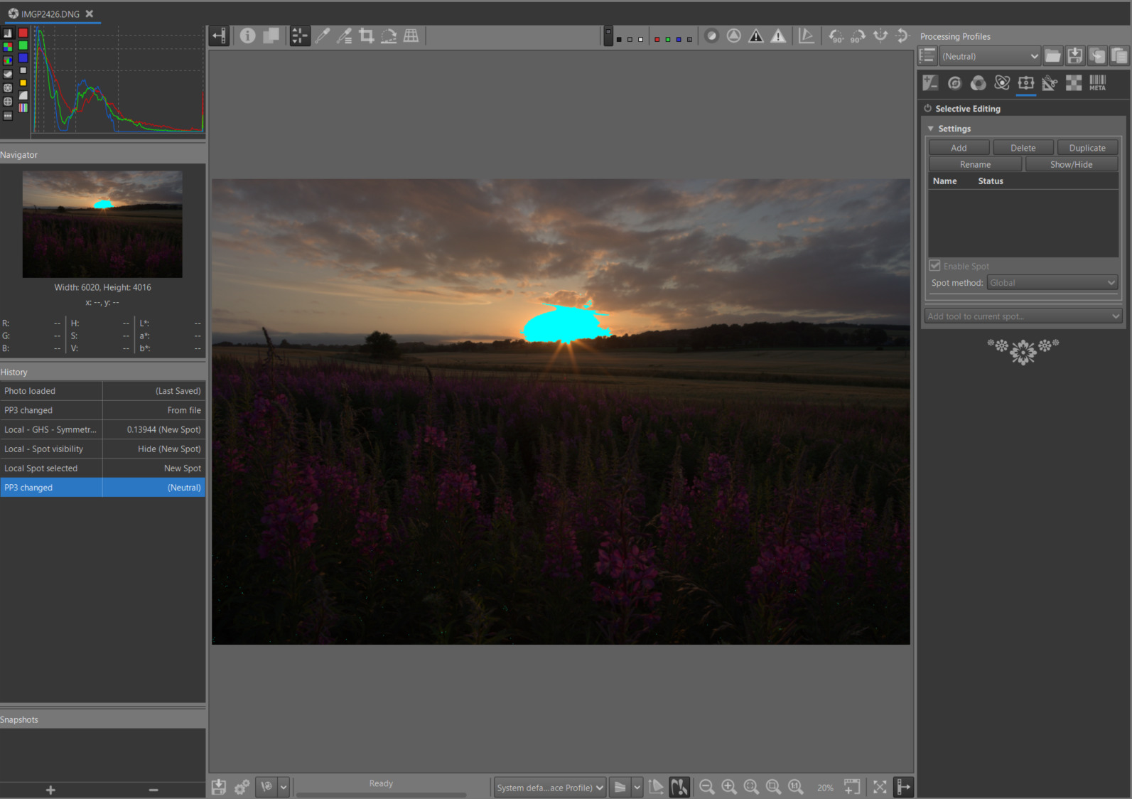
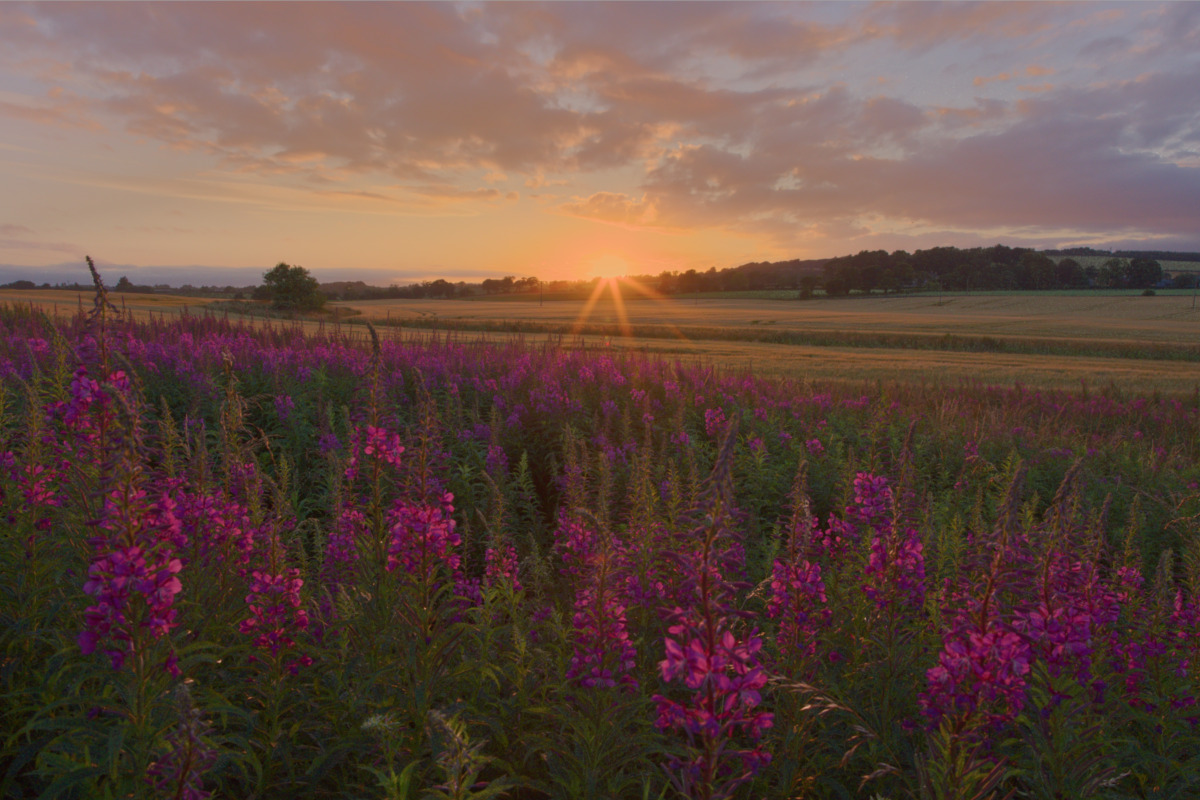
I added the ‘Michaelis-Menten’ (MM) algorithm to Selective Editing. This algorithm has the advantage of being simple for the user and is very efficient in most cases. It’s a tone mapper using the Michaelis-Menten equation, which is borrowed from biochemistry to describe enzyme kinetics .

It has the same role as GHS, that of a 'pre-tone mapper’ which prepares the work for other ‘Game changer’ tools. Of course, like GHS, it can be sufficient on its own for certain images. Schematically, it’s essentially the same as GHS (on the goals), but simpler, with slightly fewer options for (very) difficult images. In mathematical terms, comparing MM to GHS is like comparing the curriculum for the Baccalaureate exam to a Master’s degree in Mathematics. If we put ourselves in the “mission impossible” situation, the asymptotic possibilities in the highlights are superior for GHS, but at the cost of greater complexity for the user.

I created a Pull Request
Pull Request

I added this algorithm, modifying it to:

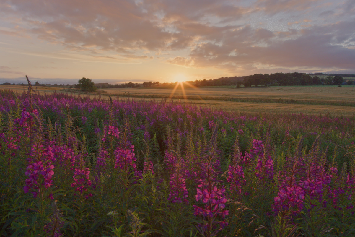
Better handling of high-dynamic-speed images, and/or poorly positioned white or black points… which is more common than you might think (even on seemingly simple images)
To easily control the highlights
Equip it with an LMS matrix that takes into account the Working profile. I had fun creating my own matrix… I added an ‘x’, for matriX.

I was inspired by the CTL from ART, thanks to Alberto…

It’s simple to design; it took me a whole day (the weather’s bad here…) to do everything…

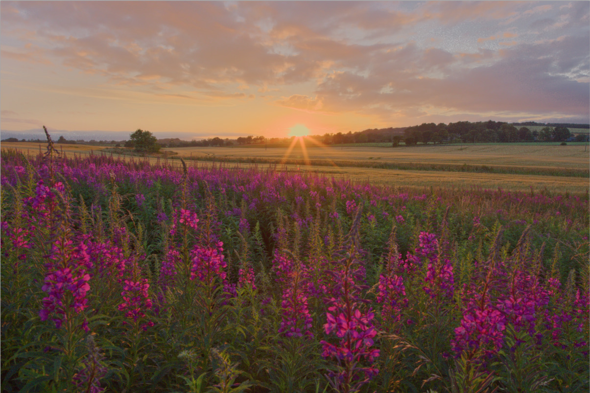
It’s easy to use, and for me, it works with the vast majority of images. Of course, it’s part of the "game changer"concept.

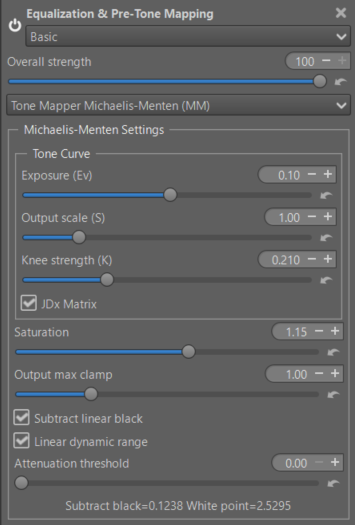
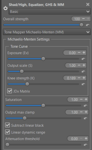
The main settings (the original ones where I haven’t changed much)

Exposure : Adjusts the input image brightness.
Output scale (S) : Controls the maximum asymptotic value of the curve; essentially the output white level.
Knee strength (K): Determines the “knee” of the curve. Lower values result in a sharper transition to the compressed highlight region.
Saturation : Adjusts color saturation post-tone mapping.
Output max clamp : Sets the final clipping point for the output values.

I haven’t added an on/off button, but that shouldn’t be a problem.

You need to pay attention to the additions I’ve made that concern :

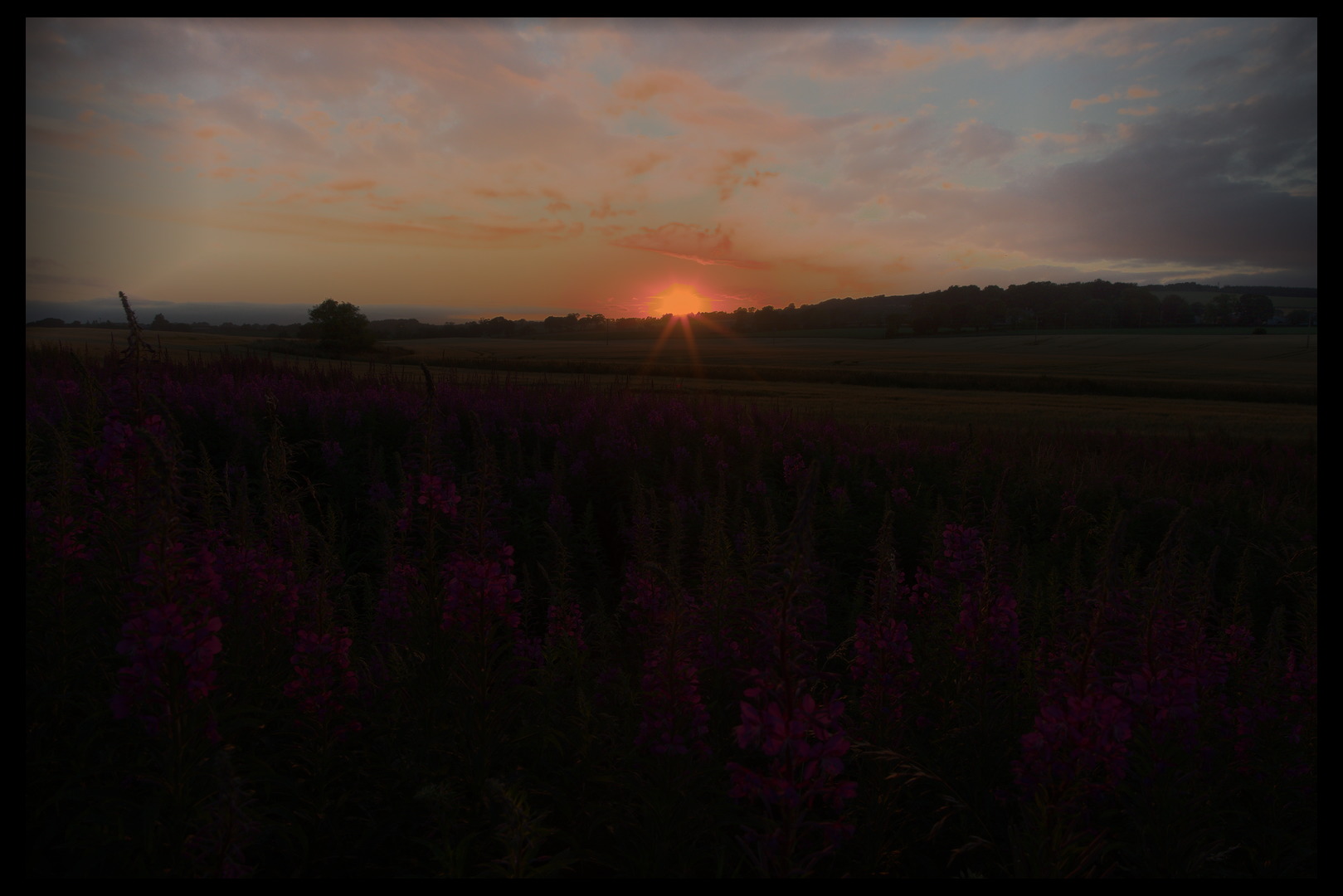
‘Subtract linear black’ and ‘Linear dynamic range’ : I emphasize the word linear. It’s the same principle as GHS: to be sure that all the data are in the interval [0 1]. If, for example, the Black Point is 0.03, it’s not 0; you lose contrast… I’m not talking about certain images where it’s 0.15. If the white point is 0.6, you limit the algorithm’s performance. If it’s greater than 1, you’ll lose the algorithm’s capabilities again. It’s highly advantageous to recover as much as possible, using ‘Highlight reconstruction > Color propagation’ (after verifying that this actually benefits the current image). The operation is very simple, at the level of a CM1 student. To simplify the interface as much as possible, I’ve only included checkboxes and no information. Of course, it’s easy (it’s just code) to change this and add sliders and two lines of information.
‘Attenuation threshold’ : with an exponentiel function, reduce the highlights that can cause a gamut overshot.
‘JDx Matrix’ : It’s a simple LMS matrix of my own design, using XYZ data, therefore independent of working profile.

I just did a review using Copilot, and I made a few adjustments
There are probably things that could be improved regarding the labels and tooltips. Any suggestions you may have would be welcome.

Executables
Michaelis-Menten

Jacques

jdc · January 28, 2026, 12:15pm

For comparison, all other settings are unchanged. I made this from pp3 in this thread.
I am not trying to establish a hierarchy of values.

New pp3
2010_MONTR_033.NEF-colmm.pp3 (19.0 KB)

Game changer : Mastery of Colors & Film simulation

Beyond the way of dealing with “hyperbolic” (or equivalent in MM) and black and white point. The two systems work differently. GHS uses the three RGB channels and an “equivalent luminance” to calculate parameters. MM uses the three RGB channels, but without relying on this concept.

There is no saturation adjustment in GHS (or only a very slight one in internal code), while MM’s saturation is achieved after an RGB-to-HSL conversion, then an HSL-to-RGB conversion.

Using lockable color pickers makes it easy to see the (small) differences and the effect of checkboxes on a standard image (Subtrack linear black, Linear dynamic range).

I made some changes to the GUI…Some titles were better suited, and some fields were removed that were not appropriate.

I just also change, saturation (internal with code), and change default setting slider saturation. The images were undersaturated by default… It’s the hyperbolic processing (basically that’s what it is) that weakens the colors.

Jacques

jdc · January 29, 2026, 7:28am

I’d like to make a few comments:

For GHS (Generalized Hyperbolic Stretch) and MM (Michaelis Merten), I use the term ‘Pre-Tone Mapping’ because, regardless of the terminology and conventions, it’s the most appropriate.

It’s placed near the beginning of the process (but not in the Raw color space), after white balance and the assignment of a Working Profile.
The goal is to control the data, particularly the black and white points, in a real-world situation. That is, at the moment of use. Of course, this won’t be able to (or will only poorly) correct Raw defects (which are rare) or poorly matched color matrices.

The objective of the GHS and MM modules is to obtain an ‘acceptable’ image that can then be processed correctly and easily. By acceptable, I mean a balanced control of shadows, highlights, contrast, exposure, and saturation. Of course, it’s possible (almost) to get it right the first time.

This is the concept of a ‘game changer’. It’s after this processing that you can fine-tune the tones, colors, contrast, etc. Of course, I recommend :

“Abstract Profile”- which, despite its somewhat esoteric name (which is precisely what it is) - can perform almost all the necessary operations: Tone balancing (using the TRC Tone Response Curve), Contrast enhancement (using ‘hidden’ wavelets), retouching of Primaries and Illuminants.
“Color Apperance & Lighting”: This often misunderstood concept incorporates the latest advances in colorimetry research (it’s not a gimmick, and it’s not as complex as it seems once you understand it). It has long used (sine 1997) the concepts of ‘scene’ (or ‘source’) and ‘viewing’ (or display). It attempts to take into account a significant number of physiological aspects, shooting conditions, and viewing conditions.

To get back to GHS and MM. It’s not one or the other, at a single moment.

You can combine 2 GHS: a) the first (in Global mode) by setting a ‘Stretch factor (D)’ strength and a ‘Local intensity (b)’ location, focusing on the shadows. The output data will be in the interval [0 1], then a second by setting a ‘Stretch factor (D)’ strength and a ‘Local intensity (b)’ location to balance the overall image.
You can combine it with another GHS: in ‘Inverse’ mode to cancel an effect or darken or reduce the contrast on a specific area, for example a sky or a sunset. In this case, it must be used with an RT-Spot in ‘Normal spot’ mode.
You can use MM as your first RT-spot - in Global mode, as it is ‘simpler’ to approach than GHS, and then continue with an ‘Inverse GHS’ to retouch a sky, or shadows, in ‘Normal spot’ mode.
etc.

Each time, you simply need to add a new RT-spot in ‘Selective Editing’.

Jacques

SCHA · January 29, 2026, 7:25pm

Merci beaucoup @jdc

I’ll certainly give this a try very soon… More learning!

I also appreciate your guidance and tutorials above.

jdc · January 30, 2026, 7:03am

Thanks @SCHA , it’s a real pleasure to receive a comment, even if I see the ‘likes’.

I regret that, unlike what happens with other free software, there’s little interaction. I’m not talking about Playraw, which maintains its personal aspect and allows for comparisons, but I’m talking about how it works, including the technical aspects.
Just one example, without directly comparing GHS and AgX: for GHS, if I exclude my own posts, there have been 100 interactions in the last year, that’s the maximum. AgX has over 3000. Well, I’m not forcing anyone, but we’re still in the realm of confidential information… Perhaps it’s the names of the algorithms, or the lack of documentation? But for me, it’s very difficult to do something without user feedback.

Good news this morning! I received a post from Pat @patdavid the migration to Hugo is progressing. I don’t know when we’ll have it, but it makes me happy… Of course, someone needs to write and implement it in Hugo…

Thank you again.

Jacques

SCHA · January 30, 2026, 8:55am

Sorry, Jacques, I deleted my post, and will try to remember the essence of it…

I know what it was… You’re very welcome

Merci beaucoup

Sunhillow · January 30, 2026, 12:45pm

You can recreate your post by clicking the pencil symbol and copying your old text.

I did not yet have time to try out this algorithm created by @jdc , but after trying your pp3 from Kiyomizu-dera it looks really promising!

jdc · January 30, 2026, 1:17pm

Here’s a comparison of a challenging image I’ve already presented: a sunset.

Raw file
IMGP2426.DNG (27.5 MB)

Why do I say challenging? If you set the image to ‘Neutral’ and enable softproofing with ‘Highlight pixels with out-of-gamut colors’ in sRGB mode… the sun is already out of gamut, and the rest of the image is very dark.

I created two pp3s, one entirely with GHS (Generalized Hyperbolic Stretch) , the second with the first spot using MM (Michaelis-Menten), and the second with GHS. I then adjusted the settings, which I won’t detail here; they are in the pp3s.

First pp3 - GHS
IMGP2426.DNG-ghs.pp3 (23.1 KB)

Second pp3 - MM + GHS
IMGP2426.DNG-MM.pp3 (20.8 KB)

The two images are screenshots taken in Photoshop (very old).
In both cases, apart from two or three pixels, there are no out-of-gamut colors.
Note the difference between the sky and the sun. Which is better, I don’t know.

In both cases, the key points to remember
GHS

set to Neutral
Exposure tab - disable Clip out-of-gamut , enable Color Propagation
Raw -tab - enable Capture Sharpening
Color Tab - White balance auto - temperature correlation - Close to full CIE diagram - note Green refinement = -0.03 to avoid artifacts in the sky
Color Tab - Gamut compression - Target compression gamut sRGB - note Roloof 0.70 and settings Threshold, to remove artifacts
Color Tab - Abstract profile - note the ‘big’ Contrast Enhancement (hiden wavelets), and of course others settings
Selective Editing - 3 RT-spots GHS - the last ‘Inverse GHS’ - I’ll let you discover the settings.
Advanced Tab - Color Appearance & Lighting - I’ll let you discover the settings.

MM + GHS

set to Neutral
Exposure tab - disable Clip out-of-gamut , enable Color Propagation
Raw -tab - enable Capture Sharpening
Color Tab - White balance auto - temperature correlation - Close to full CIE diagram - note Green refinement = -0.03 to avoid artifacts in the sky
Color Tab - Gamut compression - Target compression gamut sRGB - note Roloof 1.20 and settings Threshold, to remove artifacts
Color Tab - Abstract profile - note the ‘big’ Contrast Enhancement (hiden wavelets), and of course others settings
Selective Editing - 2 RT-spots : The first with MM - the last ‘Inverse GHS’ - I’ll let you discover the settings.
Advanced Tab - Color Appearance & Lighting - I’ll let you discover the settings.

In both cases, I pushed the settings (perhaps too far depending on your taste) to the limits of the color gamut, so that we could see the potential differences.

The executables have been updated after some GUI bugs and code optimization, plus a few other minor tweaks.
Binaries - Michaelis-Menten

Jacques

SCHA · January 30, 2026, 3:44pm

Ok… cool, thanks. Appreciate the tip, I had no idea, and was on mobile so it all went a bit downhill… Back on laptop now though!

Kurt · January 30, 2026, 3:53pm

Referring to interactions to GHS / AGX
I think the main difference lies in the amount of users. You can see it also in the amount of topics referring to DT vs RT.
But, perhaps we RT users are more satisfied with our software?

Anyway…When you will have finished your (most appreciated) work, I will gather your information, translate it in my own language,…, so that I will know when to use which tool(s) in which way. You have your enviably scientific knowledge, but despite your great tutorials, each images has its own difficulties, and still it’s some try and error for me. In the end, it’s a new, different way I must get used to.

jdc · January 30, 2026, 4:10pm

@Kurt

In fact, personally, whether one or two people make comments or suggestions, or a hundred, doesn’t bother me at all. I could even say the opposite, since it means fewer potential revisions to make. It’s simply an observation. It doesn’t keep me up at night, even though my sleep is very poor given my age and health.

Thank you

Jacques

SCHA · January 30, 2026, 4:19pm

Here’s my go at the sunset with GHS. Not managed to try MM yet… but I was pleased I managed to get the blown highlights of the sun sorted! for me… small wins!

Still some work to do on the clouds… but GHS is great! Merci @jdc

IMGP2426.jpg.out.pp3 (23.8 KB)

What I can’t work out is why my jpegs are so dark… Is it just me… What do you see when you see my jpeg? I see dark foreground, but when I edit in RT it all looks very bright.

I’ve looked at Colour Management, and my input profiles match my output (Abstract Profile; sRGB; Camera Standard)… And soft-proofing enabled…

What am I doing wrong…

Wayne_Sutton · January 30, 2026, 5:51pm

The MM + GHS version is most impressive @jdc. One thing I have found when using GHS on its own is that it is very easy to generate magenta casts in partially blown highlights that are difficult to remove (the best way I’ve found seems to be to add an MM using deltaE detection in the affected area). I get the impression that there is the same phenomenon around the sun in the GHS version above. Or is it just my imagination?

jdc · January 30, 2026, 6:10pm

@Wayne_Sutton

It is very difficult to generalize, but it is certain, even though in both cases they are hyperbolic functions.

GHS’s settings go deeper (if I can use that term). MM is simpler to use, almost instantly providing the “right” setting.

GHS allows you to use the full potential of the color gamut… even if it means producing (overly) saturated colors in highlights outside the gamut. Whereas MM naturally desaturates a lot. To prevent MM from giving the impression of a “washed-out” image, I had to significantly increase the saturation due to the difference between the luminance values before and after.

Another important point is that by default, GHS uses ‘RGB luminance’ (there are other options in the menu if you set the complexity to ‘standard’ : try ‘RGB standard’ for the 2 first Spot… Big difference), which calculates values from an equivalent luminance (similar to Lab’s ‘L’), whereas MM uses the three RGB channels separately (with the same values). I could have (but didn’t) done the same thing for MM.

But the real question is, “What happens when you go way beyond the gamut?” Anyone who can answer that is more than just an expert.

Thank you for this comment which advances knowledge, it is exactly what I was hoping for.

Jacques

jdc · January 31, 2026, 7:27am

Hello

Yesterday’s interesting exchange, with Wayne’s observation @Wayne_Sutton , allows me to make a few very simple changes to the code:

By default, GHS is now in “RGB standard” mode (similar to MM). Of course, if you previously selected RGB Luminance (which was the default), this choice will be retained via pp3. In the current situation, or for images that have already been processed and that you wish to change, you need to change the complexity mode of the RT-spot and set it to ‘Standard’. This choice (RGB Standard) is more consistent with that of MM
I changed the thresholds and luminance calculation parameters for ‘Out of gamut’ to “RGB Luminance” mode (anyone who knows what happens when the white point is 5 times or more from the “normal” maximum is a super expert). I think that for difficult cases, direct sunlight in the image, LED will be better.

Hence the importance of testing and discussion; otherwise, there’s only my arbitrary point of view… All of this was very simple to do, and does not call into question compatibility with version 5.12 (since these ‘calculation’ changes occurred after the release of 5.12). Of course, this new ‘distribution’ of thresholds for ‘RGB Luminance’ is also arbitrary; I can change it. Nevertheless, it will always be different from RGB Standard.

New binaries
Michaelis-Menten

During the day (I hope), because this morning I’m taking care of some administrative tasks; I’ll update (a new page) with the new settings.

Along with fine-tuning MM and GHS, I (slightly) improved the “Contrast enhancement” section, avoiding increasing local contrast (even though I don’t like this term which doesn’t mean much) in the highlights (This has already been done for deep shadows.)
If you would like to learn more about this algorithm, which is 99% wavelet-based, you can follow this link.
Contrast Enhancement

As a reminder, a little history. I created the first version of this algorithm in 2012. You can find it in other software. But that’s not the point.

There are a whole host of algorithms for modifying ‘local contrast’… We would first need to agree on what that is. They vary in complexity (the last one I mentioned is really complex), but they must remain simple for the user.
In RT there are a bunch of sections that deal with this, including Contrast By Detail Levels (CBDL), Wavelet Levels (for which I wrote most of the code), and others…
As I briefly explain in the link, you need to be able to increase the contrast (in the Wavelet sense of the term: that is, everywhere there is ‘depth’, whether in 2x2 pixels details or 1024x1024 pixels). If you do nothing more than adjust the contrast levels, you end up with a disaster and artifacts everywhere. Hence the algorithm conceived in 2012.
Simply put, I’ve combined the concepts of CBDL (or Wavelet Levels) with ‘Local Contrast’… You have the following in the user interface:

a slider ‘Contrast profile’ to determine the scope of what you want to do (either focusing on small details, or encompassing large 1024x1024 areas… here we’re no longer talking about “details”)
a ‘curve’ that, based on the existing local contrast, amplifies or reduces it. The ‘middle’ of the curve reflects the dominant local contrast regardless of the level of detail.

Next, there are two sliders that modify the value of the signal taken into account (generally, there’s no need to adjust them, except in special cases, for example, architecture, portraiture, etc.): ‘Attenuation response’ and ‘offset’.
Then a final one, to increase or decrease the contrast (here in the literal sense of the term, again if we agree on what it is) on the undecomposed part of the image (therefore without relief or little): Residual contrast.

This last modification is in the latest executable
Michaelis-Menten

Jacques

jdc · January 31, 2026, 1:41pm

Here, after the changes I mentioned for GHS, by default use ‘RGB standard’, and in ‘RGB Luminance’ mode change the parameters that take luminance into account in the ‘out of gamut’. I’m not posting the image with Michaelis-Menten (MM) again.

First image with GHS RGB Luminance
IMGP2426.DNG-ghs-Lum.pp3 (23.0 KB)

You may notice, among other changes, the decrease in reds (even if we like them) in the sky near the sun

Second image with GHS RGB standard
IMGP2426.DNG-ghs-std.pp3 (23.0 KB)

You will notice that it is quite similar to the one with Michaelis-Menten (MM)

Executables
Michaelis-Menten

As a reminder, as I mentioned above, I modified the ‘Abstract Profile > Contrast Enhancement’ section a bit - which can be described, although I don’t like that term, as ‘Local contrast’ (taking highlights into account… and I commented the code to make it a bit more understandable).

Thank you for your opinions and comments.

Jacques

paulmatth · January 31, 2026, 4:52pm

Bonjour Jacques, when I follow your link, I don’t see any executables there. Only tech stuff that I do not understand.

You used to place them on the page below, but the builds there are three or four weeks old.

jdc · January 31, 2026, 5:06pm

Salut Paul

No, I didn’t choose to do a pull request with that option, I could have. But the executables are in ‘GitHub > actions’… But I can do it if you want.

Jacques

jdc · February 1, 2026, 1:50pm

I added a label (and a tooltip) to ‘Michaelis-Menten’ at the bottom of the window, which allows you to see what the action on the checkboxes corresponds to : ‘Subtract linear black’ and ‘Linear dynamic range’

Executables
Michaelis-Menten

I’ve attached the tooltip (probably in bad English).

« Allows you to see the user’s action on the 2 checkboxes:

‘Subtract black’: reduces the value of the Linear Black point near to zero by subtracting the indicated value.
‘White point’: after subtracting the Black Point, divide the RGB values by the ‘Linear dynamic range’ (White point indicated value - new Black point).

Bringing the black point close to zero, and taking into account the ‘Linear dynamic range’ allows the algorithm to be optimized (better contrast, better consideration of the real gamut).
Activating ‘JDx Matrix’ will, in addition to a different color balance, reduce the ‘Linear dynamic range’ »

I’ve attached a raw file known for its poor black point quality – I intentionally didn’t use the ‘Dehaze’ checkbox in ‘Raw Black Points’ to highlight the effect of the ‘Michaelis’ checkboxes. I’ve also attached the unfinished pp3 file, for educational purposes only.
Try it with and without the checkboxes enabled, and you’ll see the differences in the settings and the image.
D200_20070802_2087-mich.NEF.pp3 (18.4 KB)

D200_20070802_2087.NEF (8.0 MB)

Some technical information. Don’t run away, I’ll reset it (I hope) simple.

Hyperbolics
Both GHS and MM use hyperbolic functions, but of a different nature. Michaelis’ function can work without problems in any data range (it’s best to put it in [0, 1]). GHS assumes the data is in [0, 1] otherwise it clips the data, which is unfortunate. This has significant consequences in terms of code and for users.

There are several types of hyperbolic functions, all sharing, despite their different mathematical principles, the common characteristic of implementing asymptotic functions that approach a value without ever reaching it (a typical example being highlights):

Those that use the usual functions ‘sinh’ , ‘cosh’, ‘tanh’, or even compositions of functions exp(x) and exp(-x). GHS falls into this category. Its distinctive feature (hence the term ‘Generalized’) is that the formula changes seamlessly depending on the settings… this is what makes it remarkable. I’ve attached the ‘Desmos’ demonstration (feel free to expand the left panel to see the formulas). But it is complex to implement and for users GHS - Desmos
Sigmoid can also be considered a hyperbolic function for the ‘highlight’ part, even if its use is more in the field of statistics or AI, basically it is a model of the normal Gaussian function.
Michaelis-Menten : this function uses the Michaelis-Menten equation, which is borrowed from biochemistry to describe enzyme kinetics. It is simple and comes in the form : (S * x) / (K + x). Where ‘S’ is ‘Output scale’ and ‘K’ is ‘Knee strength’. It has the advantage of being easy to use and gives good results, more easily than GHS. However, it is not reversible.
A similar function is used in ‘Gamma based’ and ‘Slope based’ in Selective Editing > Color Appearance (CAM16 & JzCzHz)

JDx Matrix
What is it and what is it used for? It is based on the concept of LMS using XYZ data :LMS (long, medium, short), is a color space which represents the response of the three types of cone cells of the human eyes, named for their responsivity (sensitivity) peaks at long, medium, and short wavelengths.

In practical terms, there are two possible uses :

Before processing, an LMS transformation is applied, which will modify the color dominants in that processing, and at the end, the inverse transformation is applied. Only the data from that processing will be modified.
To serve as a compressed (then decompressed) color space in CAMs (Color Appearance Models) such as CIECAM or JzCzHz. The goal here is, as with the previous model, to modify the colorimetry, but above all to allow working on a smaller color space, where one can play with imaginary colors without (too much) concern. Of course, these CAMs incorporate different methods to take into account physiological aspects and shooting conditions. This is not the case with the previous model.

JDx Matrix, is in the fisrt case. How it works ? I’m attaching part of the code.

 Matrix lms_mat = {{//JDx - Jacques Desmis Matrix XYZ -> LMS - Simple matrix that amplifies the current channel.
                    { 0.83, 0.1, 0.07 },//Red (L) predominant in LMS with a little more green
                    { 0.12, 0.78, 0.1 },//Green (M) almost neutral, with a little more red
                    { 0.11, 0.09, 0.80 }//Blue (S) almost neutral, with a little more red
                }};

As you can see, it’s a kind of table (a matrix with 9 numbers). Its use is simple. If you observe the pixels of each image, they will have (we’ll stick with a simple case) values like this for a pixel: X=0.4, Y=0.2, Z=0.7.
To obtain the value of ‘L’, we multiply the coefficients of the first line with the values X, then Y, then Z respectively, by adding them together
This will give for ‘L’ : 0.83 * 0.4 + 0.1 * 0.2 + 0.07 * 0.7 = 0.401. This value will become the new data used. We do the same for ‘M’ and ‘S’ with the second and third lines.

It is important to note that I was not referring to RGB data, but XYZ data. In 1931, researchers from the CIE (Commission Internationale de l’Eclairage – in french). They imagined a reference space to free themselves from the constraints of RGB spaces (they did this with a panel of volunteers) which led, in particular, to the CIExy diagram (the limits of human vision). It is therefore important that the matrix be independent of the Working Profile and remain the same; for example, if the user chooses ‘AdobeRGB’ instead of Rec2020, the matrix will remain the same. Of course, the RGB data must first be converted to XYZ (and vice versa).
Of course, for the user it’s completely transparent. The inverse matrix is calculated… I chose a simple matrix (there are only 2 significant numbers), giving more pleasing images and lowering (a little) the white point in out-of-gamut images.

Thank you

Jacques

SCHA · February 1, 2026, 3:33pm

IMGP2426-1.jpg.out.pp3 (21.5 KB)

Well it’s taken a long time but this is more pleasing to my eye… I struggled with the output… played around a lot, now hopefully getting somewhere.

Thanks again @jdc for your input and efforts with this module and the explanations (not that I understand very much ), but I am enjoying the ride!