G'MIC Adventure #7: Variable Density Hilbert Curve

[David_Tschumperle (G'MIC staff)]

After reading the post from @lylejk : https://discuss.pixls.us/t/variable-density-hilbert-curve
(and after finishing up the few things I had to do before diving into this), I thought it would be fun to try implementing a locally variable-density Hilbert curve effect.

And to give myself a little motivation, what could be better than doing this as part of a new episode of G’MIC Adventure?

The goal here is then to write a G’MIC command that is able to reproduce an input image with a single curve that looks like a Hilbert curve, so something like this:

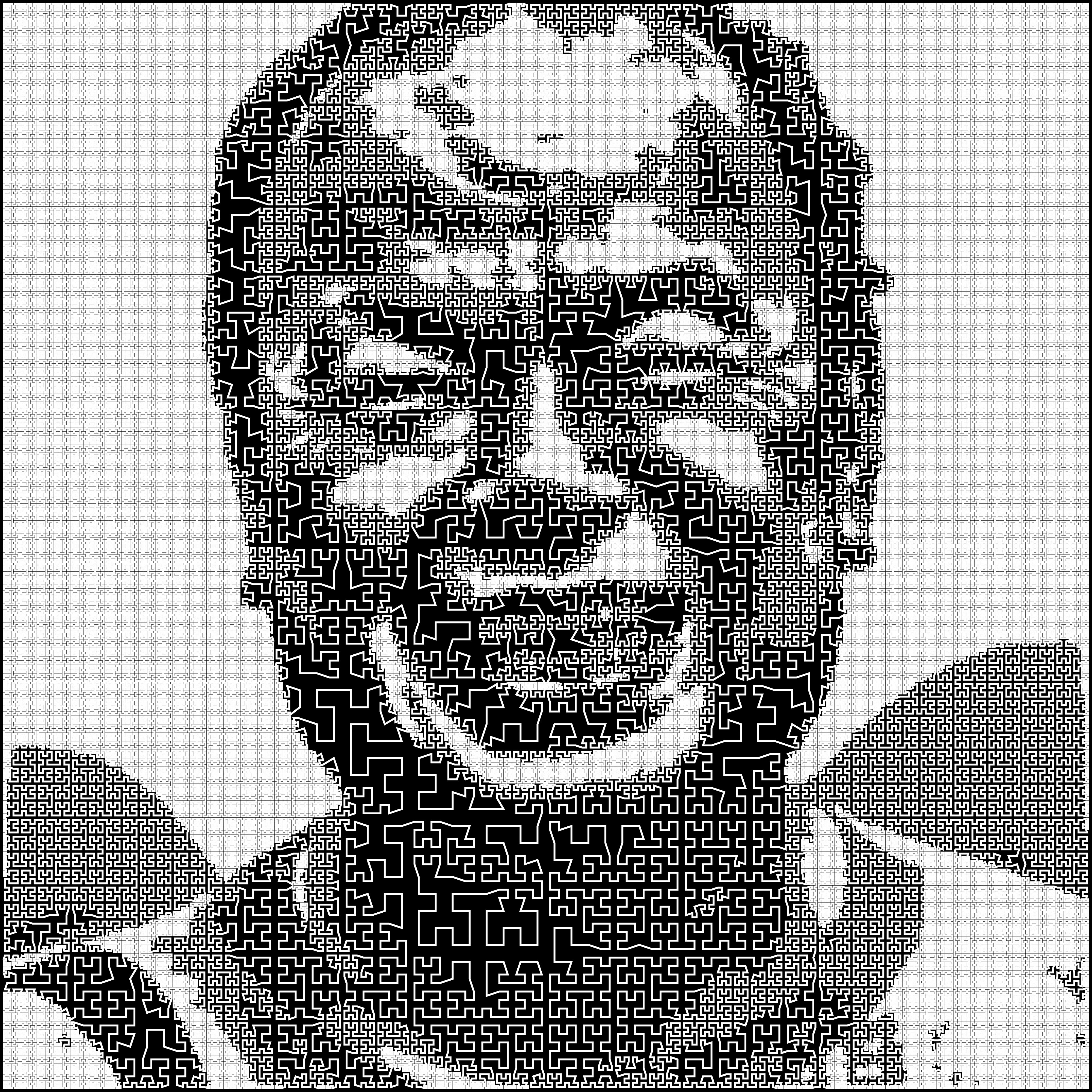
(image borrowed from the original post from @lylejk ).

That’s what I’m going to try to do here!

And since I’m naturally curious and enjoy learning new things, I’m going to avoid asking an LLM to code this for me from scratch The bad news: I have absolutely no certainty that I’ll succeed in this challenge, and it’s entirely possible that I won’t. But that’s exactly what makes it so interesting, because I’ll be able to describe the different stages of my thought process as I try to reach that result. It’s a bit like an LLM’s “chain of thought,” but much slower

---

Image analysis:

Looking at the goal image, I understand I will have to construct a single Hilbert Curve in a way that allows me to locally applies a different “subdivision deep” for the curve construction. So first, I need to understand how to construct the Hilbert curve, by iterating subdivisions and transformations.
G’MIC already has a command shape_hilbert that draws a Hilbert Curve, but it uses some fancy math tricks to get the parameterization of the curve without having to deal with explicit subdivisions.
So a good idea is to first try to re-implement a command that draws the standard Hilbert curve, but using an iterative approach.

Understanding how the Hilbert Curve can be constructed iteratively:

Looking at the wikipedia page: Hilbert curve - Wikipedia
I see we can start from a ‘U’-shaped curve, and apply 4 different geometric transformations on its vertices, to get a new “subdivided” curve that is the level-1 of recursion for the Hilbert Curve construction.

OK, OK, let’s try this!

(to be continued…)

[David_Tschumperle (G'MIC staff)]

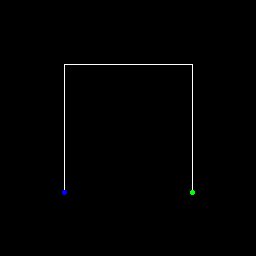
I suppose the first thing to do, then, is to draw this famous “U,” which is the starting point of the curve (we can call this “depth 0”).

Since I assume that, in the end, I’ll have to draw a single curve anyway—with a starting point and an ending point—I’m going to store my curve as a 2-channel 1D image (i.e., of size Nx1x1x2, where N is the number of points on my curve).

And I’ll start by explicitly defining my curve as a downward-facing “U” (this isn’t what the English Wikipedia page shows, but rather the French one, which—for once—seems more comprehensive to me!).

Let’s do this:

foo :
  # Init curve.
  # Vertices are assumed to be located inside the [0,1]^2 2D square, but the 'U' starts at quarter coordinates.
  (0.25^0.75,0.25^0.25,0.75^0.25,0.75^0.75) => coords

  # Visualize curve.
  256,256,1,3 => canvas
  +*[coords] 256 => normalized_coords
  eval[normalized_coords] "x>0?(P0 = J[-1]; P1 = I; polygon(#$canvas,2,P0,P1,1,255))" # Draw polyline
  circle[canvas] {normalized_coords,I[0]},2,1,0,0,255 # Draw starting point in blue
  circle[canvas] {normalized_coords,I[-1,2]},2,1,0,255,0 # Draw ending point in green
  k[canvas]

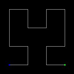
and then $ gmic foo generates this:

That’s indeed the level-0 of the Hilbert Curve ! Yipee

Now, we have to apply a set of 4 geometric transformations of this initial ‘U’ to copy/rotate/flip a version of it in each subsquare of a 2x2 subdivision of the initial [0,1]^2 square:

foo :
  # Init curve.
  # Vertices are assumed to be located inside the [0,1]^2 2D square, but the 'U' starts at quarter coordinates.
  (0.25^0.75,0.25^0.25,0.75^0.25,0.75^0.75) => coords

  # Duplicate initial curve and apply geometric transformations to get level-1 Hilbert Curve.
  +f[coords] "[ 1 - i1,2 - i0 ]" # Bottom-left quarter
  +f[coords] "[ i0,i1 ]" # Top-left quarter
  +f[coords] "[ i0 + 1,i1 ]" # Top-right quarter
  +f[coords] "[ i1 + 1,i0 + 1 ]" # Bottom-right quarter
  rm[coords] a[-4--1] x /. 2 => coords # Update coordinates

  # Visualize curve.
  256,256,1,3 => canvas
  +*[coords] 256 => normalized_coords
  eval[normalized_coords] "x>0?(P0 = J[-1]; P1 = I; polygon(#$canvas,2,P0,P1,1,255))" # Draw polyline
  circle[canvas] {normalized_coords,I[0]},2,1,0,0,255 # Draw starting point in blue
  circle[canvas] {normalized_coords,I[-1,2]},2,1,0,255,0 # Draw ending point in green
  k[canvas]

And we get:

Note that the starting point and the ending point are actually at the same locations as before, which is a good sign that the transformations we’ve just done could be iterated more than once. Let’s just add a repeat { ... } loop for the transformation part:

foo :
  # Init curve.
  # Vertices are assumed to be located inside the [0,1]^2 2D square, but the 'U' starts at quarter coordinates.
  (0.25^0.75,0.25^0.25,0.75^0.25,0.75^0.75) => coords

  # Duplicate level-n curve and apply geometric transformations to get level-(n+1) Curve.
  repeat 2 {
    +f[coords] "[ 1 - i1,2 - i0 ]" # Bottom-left quarter
    +f[coords] "[ i0,i1 ]" # Top-left quarter
    +f[coords] "[ i0 + 1,i1 ]" # Top-right quarter
    +f[coords] "[ i1 + 1,i0 + 1 ]" # Bottom-right quarter
    rm[coords] a[-4--1] x /. 2 => coords # Update coordinates
  }

  # Visualize curve.
  256,256,1,3 => canvas
  +*[coords] 256 => normalized_coords
  eval[normalized_coords] "x>0?(P0 = J[-1]; P1 = I; polygon(#$canvas,2,P0,P1,1,255))" # Draw polyline
  circle[canvas] {normalized_coords,I[0]},2,1,0,0,255 # Draw starting point in blue
  circle[canvas] {normalized_coords,I[-1,2]},2,1,0,255,0 # Draw ending point in green
  k[canvas]

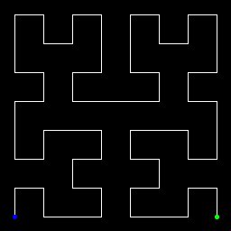
and here is the “level-2” curve:

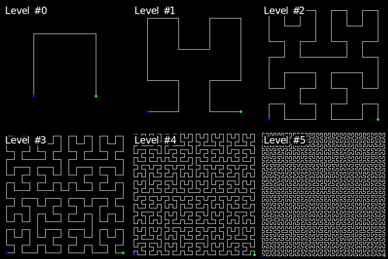
Now, if we replace the repeat 2 { ... } by an increasing number, we get the different levels of the Hilbert Curve, as expected:

It makes me realize that the more we iterate, the more “bright” the final image looks like. Keeping the overall goal in mind, it seems then relevant to try to locally decide a number of subdivision that is directly related to the luminance of the image we want to reproduce.
But that will be for a further experiment!

Next step is probably to experiment with variable subdivision, and as we clearly have a 2x2 grid decomposition at each curve level, I feel I’ll have to deal with quadtree decomposition of the image one day or another…

(to be continued…)

[Reptorian]

@David_Tschumperle

quadtree decomposition of the image one day or another…

Unrelated, but I feel you. This is one of those things where I have to figure out for packing images onto a specified dimension. Actually 3D variant.

[David_Tschumperle (G'MIC staff)]

Variable density: The lazy (and ugly) way!

Assuming we know how to build N levels of the Hilbert Curve, how can we blend them together to generate a single curve that looks like an image?

After thinking a bit about that, my idea is:

• Compute N different levels of the Hilbert-Curve (e.g. starting from a detailed-enough level, let say 3 or 4), and make sure they all have the same number of vertices (i.e. the number of vertices of the most detailed curve), using linear interpolation for lower levels.
• Then, construct a single curve from these N curves : From the starting point (which is the same for all the N-levels curves), look at the luminance of the image at that point, and decide to which curve level I should switch for the next point, regarding this luminance (quantized as N levels).
• Do the same for the next point, and construct a single set of curve coordinates.

This is what the following code does:

foo :

  # Generate N levels of the Hilbert Curve.
  (0.25^0.75,0.25^0.25,0.75^0.25,0.75^0.75) # Init curve
  repeat 8 {
    +f[-1] "[ 1 - i1,2 - i0 ]" # Bottom-left quarter
    +f[-2] "[ i0,i1 ]" # Top-left quarter
    +f[-3] "[ i0 + 1,i1 ]" # Top-right quarter
    +f[-4] "[ i1 + 1,i0 + 1 ]" # Bottom-right quarter
    a[-4--1] x /. 2
  }
  rm[0-3] # Remove first 4 levels (considered too sparse)
  r ${-max_w},1,1,2,3 a y *. 512 => coordsN # Resize all curves to have the same number of vertices

  # Draw image.
  sp portrait3,512 b. 3 luminance. quantize. {coordsN,h},0,1 => img

  # Construct the variable-density Hilbert Curve.
  {coordsN,w},1,1,2,">begin(l = 0);
    P = round(I(#$coordsN,x,l));
    l = i(#$img,P[0],P[1]);
    P"
  => coords

  # Visualize curve (animated)
  512,512,1,3 => canvas
  repeat {coords,w} {
    if $> line[canvas] {coords,[I[$>-1],I[$>]]},1,255 fi
    if !($>%100) w[canvas] fi
  }

And here is the result:

Not perfect, but not that bad for a first attempt of variable-density Hilbert Curve (and for a script with approx. 30 lines of code ).

The idea seems good enough. What is annoying is that the constructed curve seems to create intersections at the borders of different quantized areas. Maybe I can manage that in a way that is simple enough to have a nice-enough rendering. Looks like I should search for the nearest neighbor available when I do a level switch.

Anyway, at first glance, this track looks pretty good to me! I’ll try to fix these minor local glitches, but overall it already looks promising.

(to be continued…)

[Reptorian]

Yes, it does look very promising. Maybe I’ll have a crack at modifying the code to do what MadJik over paint.net forum did with his hilbert plugin.

[David_Tschumperle (G'MIC staff)]

Almost there!

So my idea of calculating lists of vertices for several levels of the Hilbert curve and merging all these curves into a single one wasn’t bad.

However, resizing all these parameterizations so that each curve would have the same number of vertices wasn’t exactly the idea of the century! That’s because I hadn’t considered the following constraint: in reality, we want to move from one level l of the curve to another (l+1 or l-1) only when we’re at a vertex of the curve at level l.

So, it makes more sense to keep the curves as they are, preserving their number of peaks. Since the curves traverse the image roughly in the same way, we can easily find correspondences between the indices of the peaks when moving from one curve to another.

So let me modify my little script so that we keep the curves at each levels as they are:

foo :

  # Generate N recursion levels of the Hilbert Curve.
  (0.25^0.75,0.25^0.25,0.75^0.25,0.75^0.75) # Level-0 curve (flipped 'U')
  repeat 8 {
    +f[-1] "[ 1 - i1,2 - i0 ]" # Bottom-left quarter
    +f[-2] "[ i0,i1 ]" # Top-left quarter
    +f[-3] "[ i0 + 1,i1 ]" # Top-right quarter
    +f[-4] "[ i1 + 1,i0 + 1 ]" # Bottom-right quarter
    a[-4--1] x /. 2
  }
  rm[0-3] # Remove first levels (too sparse)
  N=$! # Number of remaining levels

  # Quantize image to reproduce.
  sp portrait4,1024 b. 2 luminance. quantize. $N,0,1 => img

  # Generate variable-density Hilbert Curve.
  1,1,1,2
  eval "
    x = l = 0;
    while (x<w#l,
      P = [ i(#l,x,0,0,0),i(#l,x,0,0,1) ];
      da_push(P);
      nl = i(#$img,round(P[0]*w#$img),round(P[1]*h#$img));
      nl!=l?(x = int(x*w#nl/w#l); l = nl); # Find index correspondence between curves
     );
      ++x;
    ); da_freeze()"
  => coords

  # Visualize curve (animated)
  800,800 => canvas
  eval[coords] ":
    y>0?(
      P0 = J[-1]; P1 = I;
      polygon(#$canvas,2,round([ P0[0]*w#$canvas,P0[1]*h#$canvas,P1[0]*w#$canvas,P1[1]*h#$canvas ]),1,255);
    ); _0"

I’ve done some modifications to make the script adaptive to the size of the image to analyze and the size of the canvas to draw on.
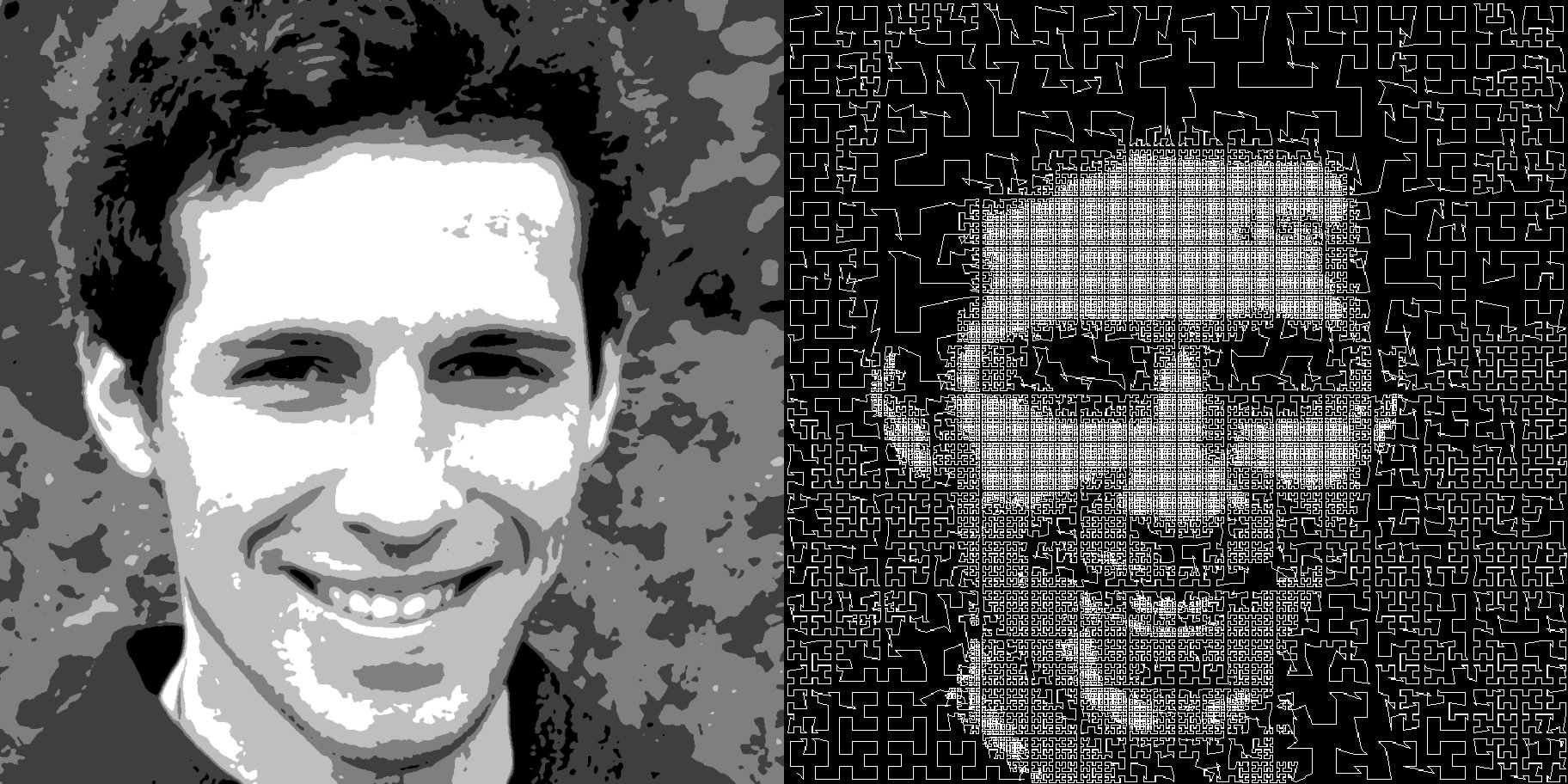
Now we obtain this (left: the quantized image, right: the generated curve)

Looks better than before!

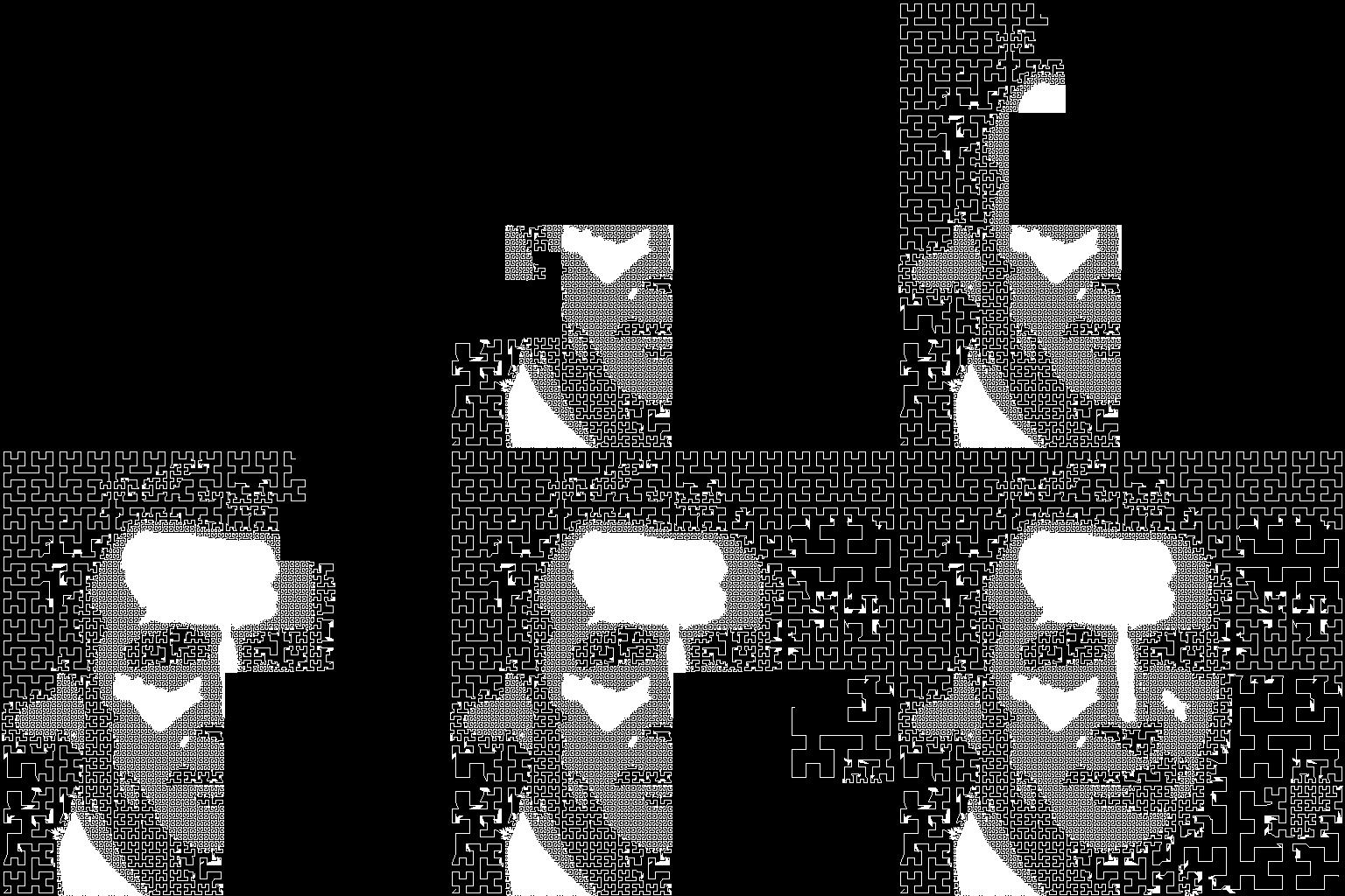
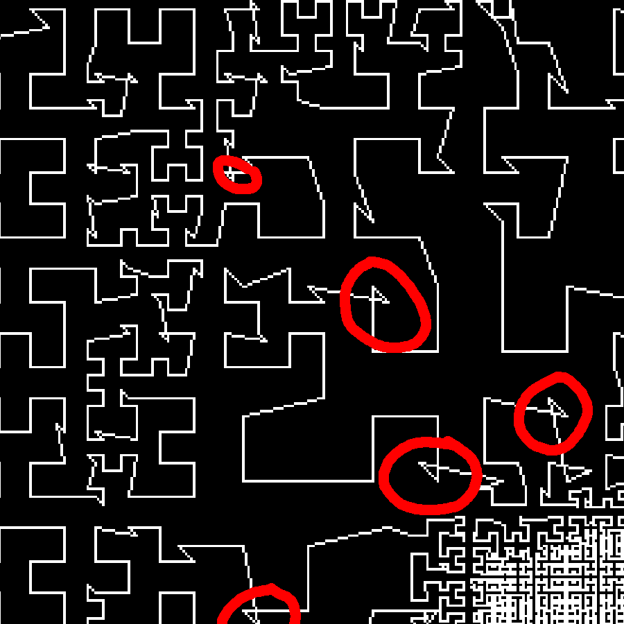
But if you look closely at the generated curve, you’ll notice a troublesome issue: the curve intersects itself, which is not the case in the example from Lylejk’s post.
Let me show you a zoom on a region to illustrate the problem:

So my next post will be about trying to solve this issue.
But as the title said: We’ve almost there!

(to be continued…)

[David_Tschumperle (G'MIC staff)]

Tweak it all!

If we go back to the explanation of how the Hilbert curve is constructed (my second post), we recall that the curve is constructed “cell by cell” (by subdividing the square into a 2x2 grid each time).

And in my code, I allow the curve to jump from one level to another even when I’m located at a point inside a cell—that is, neither at the cell’s starting point nor its ending point. That’s the mistake! It seems more logical to allow the curve to jump to another level only when we’re located at an entry or exit point of a cell. Since there are always 4 points in a cell, this is an easy constraint to incorporate into our code: we jump to another level only when (x % 4) == 0.

And here I have to admit that there’s something I don’t quite understand: Experimentally, we find that it’s actually sufficient to allow level jumps only when the index of the vertex of a curve is even, that is, (x % 2) == 0. If anyone has a geometric explanation to share, I’d love to hear it!

It also seems like a good idea to limit level jumps to the level directly above or below (but not allow jumping two levels at once, for example).
Again, this is a constraint that we can easily add to our code.

So here’s how it turns out:

foo :

  # Generate N recursion levels of the Hilbert Curve.
  (0.25^0.75,0.25^0.25,0.75^0.25,0.75^0.75) # Level-0 curve (flipped 'U')
  repeat 8 {
    +f[-1] "[ 1 - i1,2 - i0 ]" # Bottom-left quarter
    +f[-2] "[ i0,i1 ]" # Top-left quarter
    +f[-3] "[ i0 + 1,i1 ]" # Top-right quarter
    +f[-4] "[ i1 + 1,i0 + 1 ]" # Bottom-right quarter
    a[-4--1] x /. 2
  }
  rm[0-3] # Remove first levels (too sparse)
  N=$! # Number of remaining levels

  # Quantize image to reproduce.
  sp portrait4,1024 b. 1 luminance. quantize. $N,0,1 => img

  # Generate variable-density Hilbert Curve.
  1,1,1,2
  eval "
    x = l = 0;
    while (x<w#l,
      P = [ i(#l,x,0,0,0),i(#l,x,0,0,1) ];
      da_push(P);
      !(x%2)?( # Wait for a starting or ending vertex in a cell
        nl = i(#$img,round(P[0]*w#$img),round(P[1]*h#$img));
        nl>l?(nl = l + 1):nl<l?(nl = l - 1); # Only jump one level up or down
        nl!=l?(x = int(x*w#nl/w#l); l = nl);
      );
      ++x;
    ); da_freeze()"
  => coords

  # Visualize curve (animated)
  800,800 => canvas
  eval[coords] ":
    y>0?(
      P0 = J[-1]; P1 = I;
      polygon(#$canvas,2,round([ P0[0]*w#$canvas,P0[1]*h#$canvas,P1[0]*w#$canvas,P1[1]*h#$canvas ]),1,255);
    ); _0"

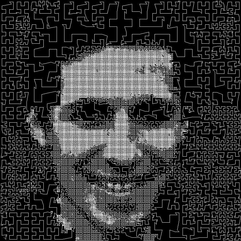
And here’s the result:

And, at first glance, we don’t have any more self-intersection problems! Good job!

So, at this point, I think the goal of this G’MIC Adventure has been achieved.
We now have a solid, simple code base that can likely be developed further as a filter for the G’MIC-Qt plugin. I’ll try to work on it if I can find some time
But the hardest part is done!

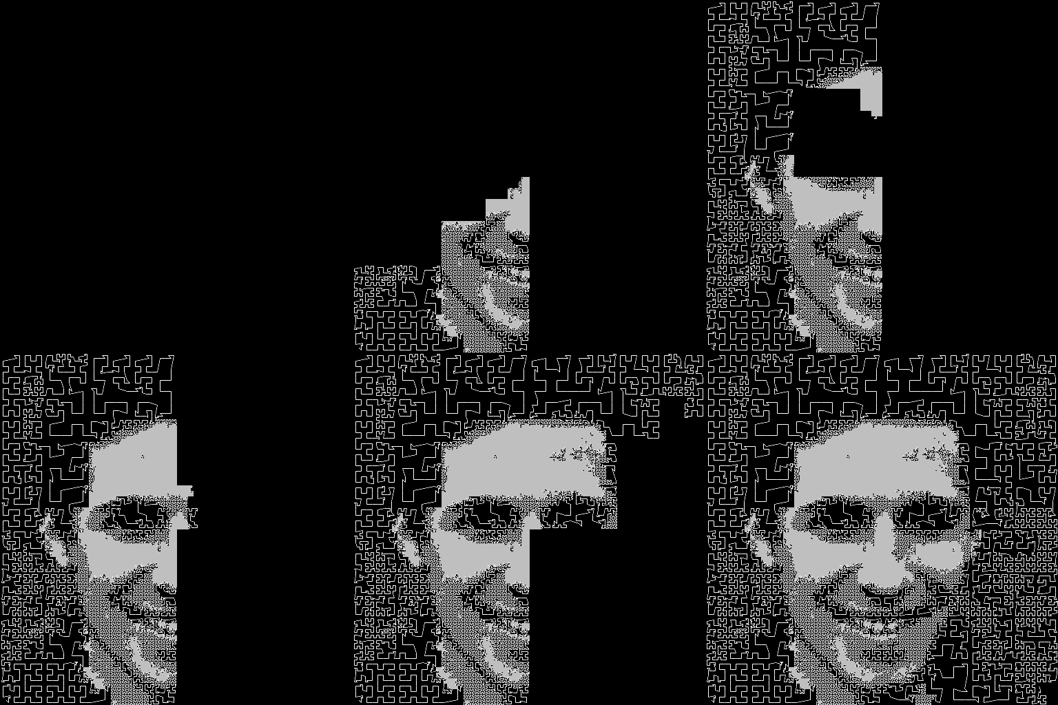
And to wrap things up, I’m sharing this short animation that shows the path of the Hilbert curve with variable density, from the bottom left to the bottom right.

I’m glad I didn’t have to explicitly build a quadtree I’ll let you know if I manage to create a filter specifically for this purpose for the G’MIC-Qt plugin.

Until then, have a great evening and good night!

[lylejk (Lyle Kroll)]

Saw this at work earlier, David and kept up with the progress between dead-time. Fantastic for sure. Hopefully, you’ll port it into the G’MIC GIMP plugin, too.

[David_Tschumperle (G'MIC staff)]

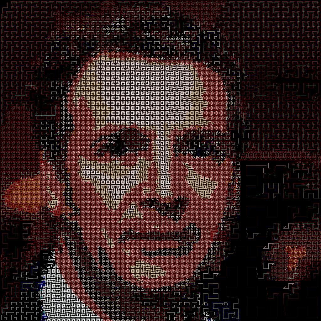
An interesting variation : Variable Density Hilbert Curve applied on each R,G,B channel of a color image, independently (each channel is then a binary image, with value 0 or 255).

[lylejk (Lyle Kroll)]

Even better. Again, hopefully the GIMP G’MIC preset will be available, soon.

[David_Tschumperle (G'MIC staff)]

I’ve finally made a filter for the G’MIC-Qt plug-in!

It’s quite basic for now, but it does the job. Not sure I will implement additional features, that will depend on whether I have time or not.

[lylejk (Lyle Kroll)]

Yes; happy camper I am, David. Saw this at work, earlier. G’MIC continues to be the gift that keeps on giving.

[lylejk (Lyle Kroll)]

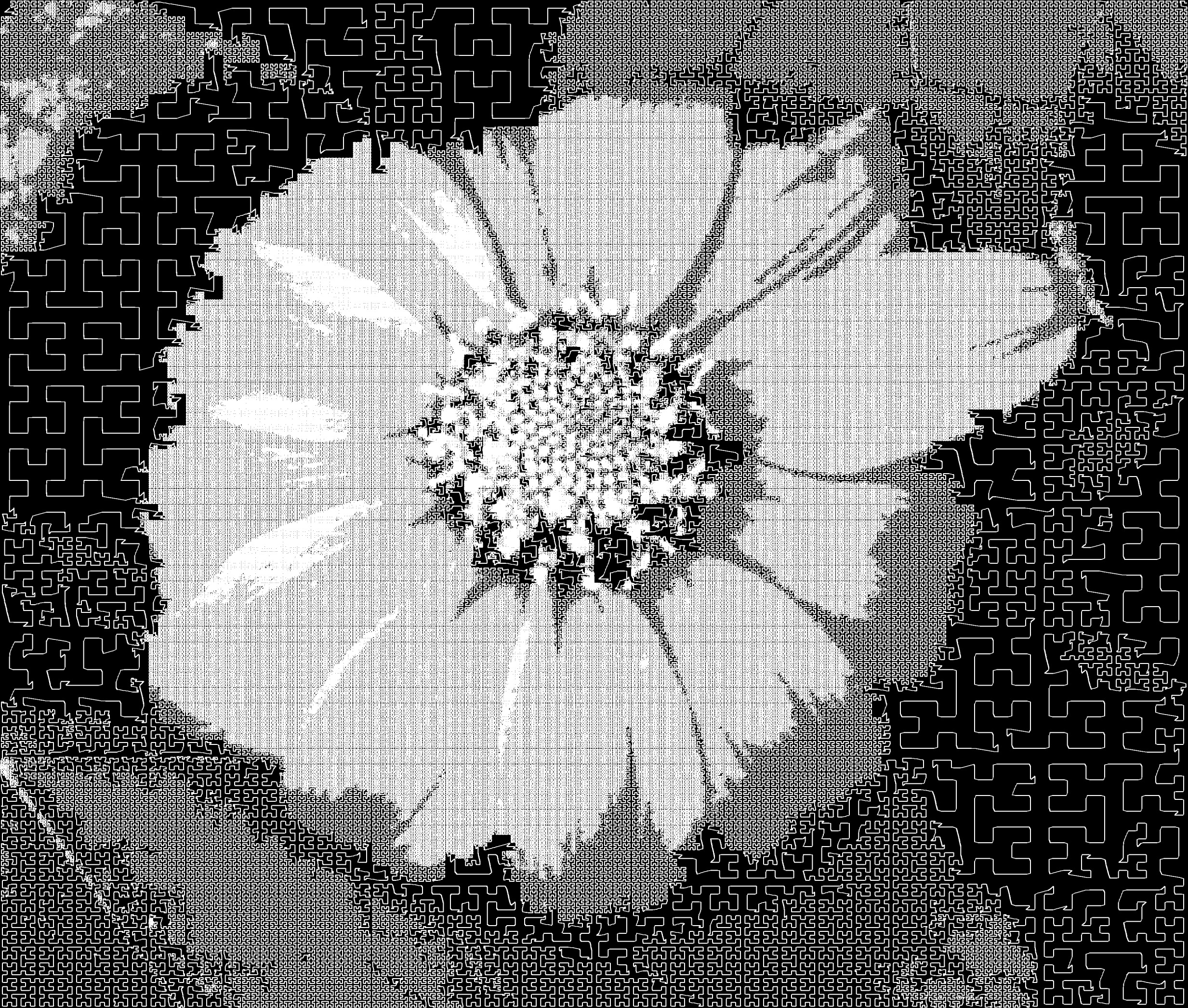
Took the picture of this Tithonia a few years back. Cropped and fed it in to the G’MIC preset for a test. I did try to do the same for my boy (cat) but just didn’t look right; not enough contrast.

[lylejk (Lyle Kroll)]

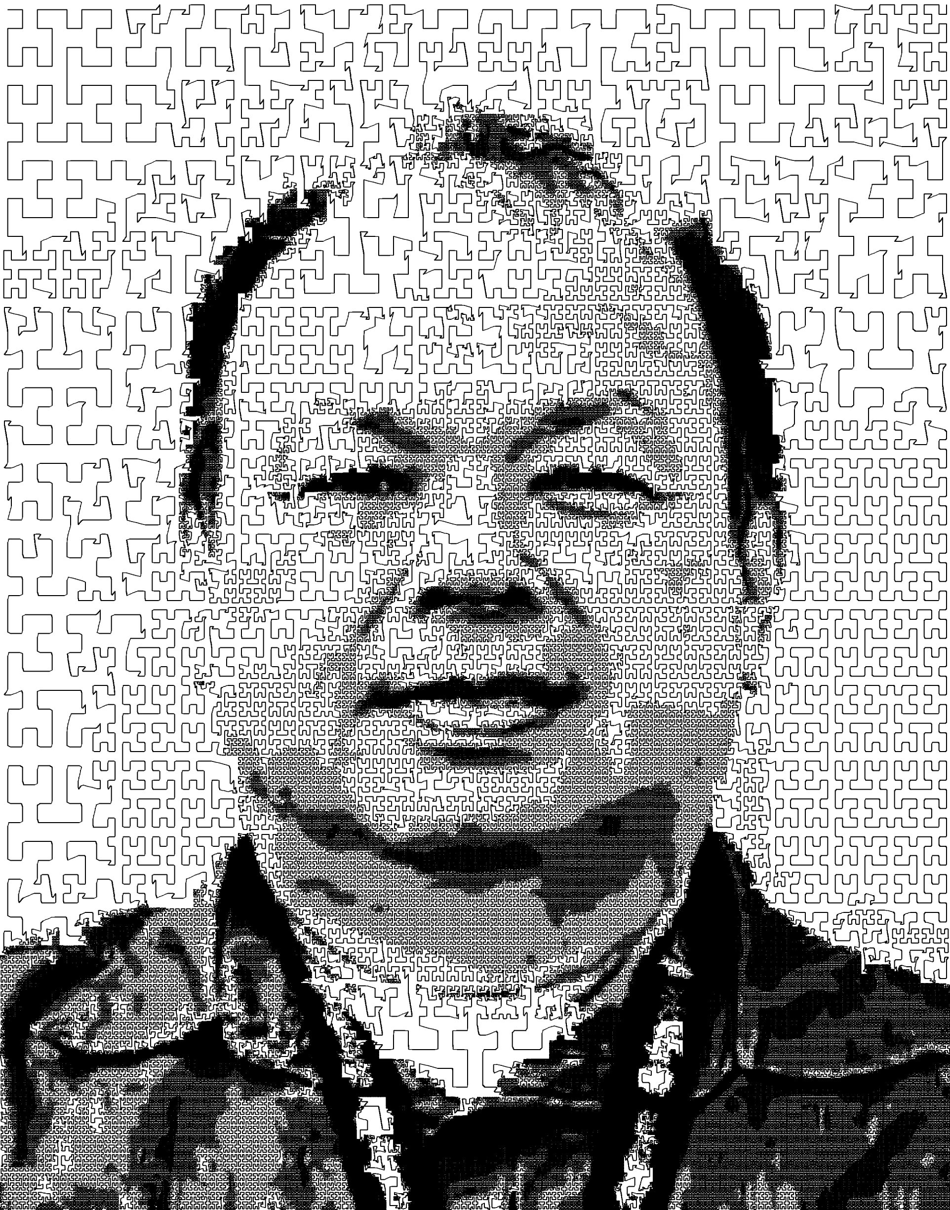
Thought I would try to scare you folk, too. lol