Today, I’d like to start a third episode of my G’MIC Adventures serie, with a quick exploration of Diffusion-Limited Aggregation: How to implement it as G’MIC scripts, and what cool things can be derived from it?
Ok, so first, what is Diffusion-Limited Aggregation ? @Reptorian already implemented it inside G’MIC a few years ago, so that’s something you may be already familiar with. But for this episode, I’m gonna re-implement it from scratch, for educational purposes (and for fun, let’s not kid ourselves ![]() ).
).
First, let me just copy/paste what Wikipedia tells about it:
Diffusion-limited aggregation (DLA) is the process whereby particles undergoing a random walk due to Brownian motion cluster together to form aggregates of such particles.
In practice, how does it translate with discrete images ? Basically, you start from an image where only a few pixels are set (e.g. with value 255, all others pixels are 0). For instance, let’s start with this simple circle outline:
dla:
  400,400 => img

  # Populate image with some points.
  circle[img] 50%,50%,100,1,0xFFFFFFFF,255

Now, the principle of DLA is as follows: You pick the location of a random black pixel in this image, and you start moving a “particle” from here under a Brownian motion (basically a completely random trajectory). And you move this particle until it collides with one of the existing white pixel of the image. When it happens, you set the latest non-colliding pixel to 255 and you start again.
Simple, right?
Here’s a simple documented G’MIC code that does exactly that:
dla :
  400,400 => img

  # Populate image with some points.
  circle[img] 50%,50%,100,1,0xFFFFFFFF,255

  # Propagate points by DLA.
  eval "
    repeat (30000,it,  # Number of new pixels we want to add

      # Find a random 'empty' location.
      do (P = [ v(w#$img - 1), v(h#$img - 1) ], i(#$img,P));

      # Compute brownian motion until a collision occurs.
      repeat (inf,
        nP = P + v([-1,-1],[1,1]);  # Choose a random neighbor
        nP[0]%=w#$img; # Make sure it does not go out of image
        nP[1]%=h#$img;
        i(#$img,nP)?break(); # Collision? Stop!
        P = nP;
      );
      i(#$img,P) = 255; # Set latest empty pixel to white
      !(it%100)?run('w[img]');
    )"
And here is how the image evolve over time when you run this script:

What’s nice about DLA is that it creates a kind of “branching” effect, as new particles tend to stick more likely to the edges of existing structures.
Now, let’s talk about some issue of this approach : You can imagine that when you don’t have many points that are already set (e.g. an image with a single point at the center), the probability that a new thrown particle collides with an existing point may become really low. It’s something we can easily verify by replacing the line
circle[img] 50%,50%,100,1,0xFFFFFFFF,255
with
=[img] 255,50%,50% # Set only a central point
We get this nice image:
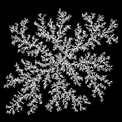
but it takes
24s of computation time, just for a 400x400 image!(for comparison, it takes only
7.5s with the circle outline).
This is a real problem, and if we want to generate larger images in reasonable time in the future, we’re going to have to find something more efficient.
And that’ll be the aim of my second post on this subject! Stay tuned! ![]()


