G'MIC Adventures #4: Physarum Transport Networks

Hello there.

I’ve stumbled across this webpage today : Algorithms for making interesting organic simulations
(thanks to the retoot of totetmatt on Mastodon!) and that looks soooo cool that I’ve decided to give a try implementing it with in G’MIC. Looks like a good candidate for a new G’MIC Adventures episode, right ? :wink:

This will be a good opportunity to see if G’MIC can easily manage millions of particles at the same time fast enough (without a GPU, I must admit I’m relying a little on multi-threaded CPU calculation!). I imagine that if it ends up working, it’ll give us the opportunity to have a new texture generation filter to offer the community!

The basic algorithm looks simple enough to implement, so I’ll start with that, and then we’ll see if we can come up with more complex variants with more parameters.
The visual results (follow the first link to see them) look amazing, so it’s very exciting to get into this!
I’m just a little worried that it might take a while to compute in an interpreted language like G’MIC. But we’ll see!

2 Likes

Iteration #1:

Well, let’s start with something simple for today.
I’ve tried to implement the very basic algorithm, as a G’MIC script, and it somehow works, at least it does produce something interesting (here, with 1M particles).
Computation time is OK on my machine, as it takes advantage of multiple cores (20 cores for me).

anim_agents-ezgif.com-optimize

I’ll probably go deeper in the experiments later, but here is my first attempt:

foo :
  400,400 => trail
  . => canvas
  1000,1000,1,3,"[ u(w#$trail - 1),u(h#$trail - 1),u(360) ]" => agents

  sensor_distance=6
  sensor_angle=45
  rotation_angle=30
  move_distance=3

  repeat inf {
    f[canvas] 0
    f[agents] ":
      const boundary_conditions = 2;
      const sd = $sensor_distance;
      const sa = $sensor_angle;
      const ra = $rotation_angle;
      const md = $move_distance;

      A = I;
      X = A[0,2];
      ang = A[2];

      Xc = round(X + sd*cexp([0,ang°]));
      Tc = i(#$trail,Xc);
      Xl = round(X + sd*cexp([0,(ang - sa)°]));
      Tl = i(#$trail,Xl);
      Xr = round(X + sd*cexp([0,(ang + sa)°]));
      Tr = i(#$trail,Xr);

      M = argmax(Tc,Tl,Tr);
      m = argmin(Tc,Tl,Tr);

      m==0?( # Lowest value straight ahead -> Turn randomly
        ang+=(u<0.5?-ra:ra);
      ):M==1?( # Highest value left -> Turn left
        ang-=ra;
      ):M==2?( # Highest value right -> Turn right
        ang+=ra;
      ); # Otherwise, no change

      ang%=360;
      X+=md*cexp([0,ang°]);
      X[0]%=w#$trail;
      X[1]%=h#$trail;
      iX = round(X);

      ++i(#$trail,iX);
      i(#$canvas,iX) = lerp(i(#$canvas,X),255,0.2);
      [ X,ang ]"

    b[trail] 0.75,2 *[trail] 0.75
    if !($>%2) +map[canvas] hot w. -1,-1,0 rm. fi
  }

Stay tuned!

3 Likes

Iteration #2:

Not too much novelty compared to iteration #1, but quite different result. What I’ve done:

  • Draw agents as ellipses rather than single pixels.
  • Try different things (simple operations) to “perturb” a bit the trail map, and get a more “organic” outcome.

I’ve played a bit with the parameters, and I got this result, which is pretty cool (I think :slight_smile: ).

A quite nice fireworks effect, that falls on the very day of France’s national holiday :wink: :fr:

Here is the updated source code, if you want to play with it:

foo :
  800,800 => trail
  . => canvas
  500,500,1,3,"[ u(w#$trail - 1),u(h#$trail - 1),u(360) ]" => agents

  sensor_distance=12
  sensor_angle=45
  rotation_angle=30
  move_distance=7

  do {
    f[canvas] 0
    f[agents] ":
      const boundary_conditions = 2;
      const sd = $sensor_distance;
      const sa = $sensor_angle;
      const ra = $rotation_angle;
      const md = $move_distance;

      A = I;
      X = A[0,2];
      ang = A[2];

      Xc = round(X + sd*cexp([0,ang°]));
      Tc = i(#$trail,Xc);
      Xl = round(X + sd*cexp([0,(ang - sa)°]));
      Tl = i(#$trail,Xl);
      Xr = round(X + sd*cexp([0,(ang + sa)°]));
      Tr = i(#$trail,Xr);

      M = argmax(Tc,Tl,Tr);
      m = argmin(Tc,Tl,Tr);

      m==0?( # Lowest value straight ahead -> Turn randomly
        ang+=(u<0.5?-ra:ra);
      ):M==1?( # Highest value left -> Turn left
        ang-=ra;
      ):M==2?( # Highest value right -> Turn right
        ang+=ra;
      ); # Otherwise, no change

      ang%=360;
      X+=md*cexp([0,ang°]);
      iX = round(X);

      ++i(#$trail,iX);
      ellipse(#$canvas,iX,4,1,ang°,0.2,255);

      [ X,ang ]"

    smooth[trail] 50,0,1,2,6
    b[trail] 3,2
    deform[trail] 2
    n[trail] 0,512

    if !($>%1)
      +map[canvas] hot
      w. -1,-1,0
      rm.
    fi
  } while {*}
1 Like

this looks so cool! this original physarium code looks great, too. interactive and with gamepad control? too bad it requires me to download some gigabyte of framework code… not sure i’ll manage.

1 Like

Amazing. Please add this scripts to g’mic with modular parameters

Iteration #3: The dance of fire!

  • Converted code to deal with a velocity vector for each agent (not specified as an angle).
  • Allowed more than 3 sensor/move orientations for each agent.
  • Added moment in velocity vector.
  • Tweaked the parameters a bit :wink:

Here is my result, that looks like a dance of fire:

Here is the updated source code:

foo :
  600,600 => trail
  . => canvas
  300,300,1,4,"[ u(w#$trail - 1),u(h#$trail - 1),unitnorm([g,g]) ]" => agents

  sensor_orientations=5
  sensor_distance=12
  sensor_angle=45

  move_orientations=5
  move_distance=5
  move_angle=30

  do {
    f[canvas] 0
    f[agents] ":begin(
        const so = $sensor_orientations;
        const sd = $sensor_distance;
        const sa = $sensor_angle;
        const mo = $move_orientations;
        const md = $move_distance;
        const ma = $move_angle;

        # Pre-compute rotation matrices.
        sRs = vector(#4*so);
        off = 0; repeat (so,k, ang = lerp(-sa,sa,k/(so - 1)); copy(sRs[off],rot(ang°)); off+=4);
        mRs = vector(#4*so);
        off = 0; repeat (mo,k, ang = lerp(-ma,ma,k/(mo - 1)); copy(mRs[off],rot(ang°)); off+=4);
      );

      A = I; X = A[0,2]; U = A[2,2];

      # Get sensor information.
      max_orientation = max_value = -inf;
      repeat (so,k,
        R = sRs[4*k,4];
        sX = round(X + sd*mul(R,U));
        value = i(#$trail,sX,1,2);
        value>max_value?(max_value = value; max_orientation = k);
      );

      # Turn agent according to sensor measure.
      max_orientation = round(max_orientation*(mo - 1)/(so - 1));
      R = mRs[4*max_orientation,4];
      U = lerp(U,mul(R,U),0.2);

      # Move agent along new orientation.
      X+=md*U;
      X[0]%=w#$trail;
      X[1]%=h#$trail;
      iX = round(X);

      ++i(#$trail,iX);
      ang = atan2(U[1],U[0]);
      ellipse(#$canvas,iX,4,1,ang,0.2,255);

      [ X,unitnorm(U) ]"

    b[trail] 2,2
    deform[trail] 2
    n[trail] 0,10

    if !($>%1)
      +map[canvas] hot
      w. -1,-1,0
      rm.
    fi
  } while {*}" && "!{*,ESC}

I like the trail version instead of canvas. But, canvas is good too.

Iteration #4: The G’MIC-Qt Filter

Well, I’ve been experimenting a lot, trying to add parameters, some of which turned out to be useless, other rendering just mess.
I think I’ve pretty much done with the basic algorithm, and I don’t really feel like going much further (I’ll be back to work tomorrow :slight_smile: ).
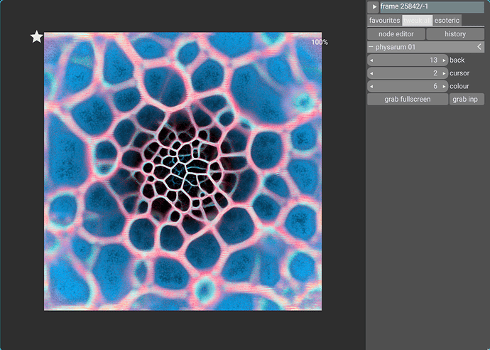
So to end the day, I compiled all this into a new filter for G’MIC-Qt, called “Patterns / Organic Fibers”, that looks like this:

Hopefully, this will be useful for some users !
Ready for testing, for users of the version 3.6.0_pre of G’MIC.

I’m tempted to say that this concludes episode #4 of “G’MIC Adventures”, but I may try something before I go to bed :slight_smile:

1 Like

I’ll give a guess. Making a mask, and generated the guided result?

Nope, but doing it in 3D.
Preliminary result:

1 Like

Would it be possible to get the something similar to fluid/smoke and acrylic splatter simulation? Not as exact but as association.


This is precisely why one should learn to code. And yes, that is possible. Actually, I might have a idea on how to do this. Draw onto image, and accumulate the frames in that image, and you should have something like that.

Tried the script versions and they’re indeed a nice way to warm up the house :slight_smile:
Played with the vars and quickly ended up with some bullet hell shmup:

PS: sorry for the bad compression… It’s actually beautiful in real time :open_mouth:

2 Likes

Iteration #5: Doing it in 3D!

As the basic algorithm was quite simple to implement, I wondered if it couldn’t be easily adapted to 3D: instead of drawing pixels in a 2D image, why not draw voxels in a 3D (discrete) image?

In the end, it took a bit more work than expected (as usual!), because to convert the algorithm to 3D, I had to :

  • Implement the drawing of 3D Gaussians oriented by any 3D vector (which is definitely harder than doing it in 2D!).
  • Adapt the sensor measures in 3D, by scanning at different voxels that belongs to the 3D plane that is orthogonal to each agent’s orientation. I had to do a bit of geometry on paper again (it’s been a long time TBH!).
  • Write a code to render the 3D volumetric image (which is dense by definition), as a 3D mesh object that renders ‘nicely’ (I used some rendering + smoothing tricks, thanks G’MIC to already have so many different smoothing algorithms implemented!).

And finally, this is what I get:

It’s not that beautiful, but before all, I wanted to test if the algorithm can be extended to 3D. The answer is yes, and I’ll be able to go to bed tonight having learned something, even if I don’t explore this 3D aspect any further!

This time, that really closes this G’MIC Adventures episode :wink:

foo :
  100,100,100 => canvas
  100%,100%,100% => trail
  40%,40%,40%,6,"[ u(w#$trail - 1),u(h#$trail - 1),u(d#$trail - 1),unitnorm([g,g,g]) ]" => agents
  w[canvas] ${"fitscreen [canvas],35%"}

  visu_ang=0
  nb_orientations=3

  sensor_distance=10
  sensor_angle=30

  motion_distance=3
  motion_angle=30
  motion_moment=0.7

  opacity=0.3

  # Define header for math expression.
  header="
    const no = $nb_orientations;
    const sd = $sensor_distance;
    const sa = $sensor_angle;
    const md = $motion_distance;
    const ma = $motion_angle;
    const mm = $motion_moment;
    const opacity = $opacity;"

  # Generate frames.
  repeat 400 {
    e " - "{_round($%*100)}%
    f[canvas] 0
    f[agents] :${header}"
      draw_gaussian3d(ind,xc,yc,zc,u,v,w,siz,anisotropy,opacity) = (
        unref(dg3d_mask,dg3d_one,dg3d_isiz2);
        dg3d_vU = [ u,v,w ];
        dg3d_vUvUt = mul(dg3d_vU,dg3d_vU,3);
        dg3d_T = invert(dg3d_vUvUt + max(0.025,1 - sqrt(anisotropy))*(eye(3) - dg3d_vUvUt));
        dg3d_expr = string('T = [',v2s(dg3d_T),']; X = ([ x,y,z ] - siz/2)/siz; exp(-12*dot(X,T*X))');
        dg3d_mask = expr(dg3d_expr,siz,siz,siz);
        dg3d_one = vector(#size(dg3d_mask),1);
        const dg3d_isiz2 = int(siz/2);
        draw(#ind,dg3d_one,xc - dg3d_isiz2,yc - dg3d_isiz2,zc - dg3d_isiz2,siz,siz,siz,opacity,dg3d_mask);
      );

      A = I; X = A[0,3]; U = A[3,3];

      # Get sensor measures.
      Y = X + sd*U;
      V = unitnorm(cross(U,[g,g,g]));
      max_value = -inf; max_Z = [ 0,0,0 ];
      repeat (no,k,
        l = lerp(0,sd*tan(sa°),k/(no - 1));
        Z = Y + l*V;
        R = rot(U,36°);
        repeat (10,a,
          value = i(#$trail,Z,1,2);
          value>max_value?(max_value = value; max_Z = Z);
          Z = Y + R*(Z - Y);
        );
      );

      # Turn agent according to sensor measure.
      U = unitnorm(lerp(U,unitnorm(max_Z - X),mm));

      # Move agent along new orientation.
      X+=md*U;
      X[0]%=w#$trail;
      X[1]%=h#$trail;
      X[2]%=d#$trail;
      iX = round(X);

      ++i(#$trail,iX);
      draw_gaussian3d(#$canvas,iX[0],iX[1],iX[2],U[0],U[1],U[2],9,0.8,opacity);
      [ X,U ]"

    b[trail] 1,2
    n[trail] 0,1

    +render_in_3d[canvas] $visu_ang on. frame.png,$> rm. visu_ang+=2

    if !{*}" || "{*,ESC} break fi
  }
  k[canvas]


render_in_3d :
  foreach {
    +ge. 0.1 * * 255 pointcloud3d
    s3d +r.. 1,{-2,h/3},1,1 /. 300 j.. . rm.
    a y
    circles3d 1.5

    -3d. 50,50,50 r3d. 1,1,1,75 *3d. 0.5  f3d 1200
    r3d. 0,1,0,$1

    1024,1024,1,3
    *3d.. 15 j3d. ..,50%,50% k.
    rolling_guidance. 4,10,0.5
    smooth. 100,0.3,1,2,5
    n. 0,255 map. hot
    rs 50%

    w. ${"fitscreen .,35%"}
  }
1 Like

@David_Tschumperle Creative application! If you made it a sphere, it could look like a tumbleweed. If you reversed the animation for the sphere, it could be an explosion. If you rotated the sphere, it could be a magical fireball. So many possibilities!

As for iteration #4, it reminds me of your spaghetti adventure. The second image reminds me of cell-like structures; if we fill it with something, it may be more apparent.

Forgot to add something about the gui version: you might want to add some code to tame the randomizer die button as half of the time i got a fully yellow or black image when using it. Or maybe just disable the particle size and opacity randomizer?

1 Like

Decided to try the 3D simulation on a bigger volume (here 400^3).
Took a part of the night to compute :wink: but the result is great !

2 Likes