Guiding laplacians to restore clipped highlights

OpenCL kernels available today.

I may have fixed this in https://github.com/darktable-org/darktable/pull/10711/commits/659782c84bff33ff5b1af7a315351332093445dd, where I choose the best guiding candidate channel with variance analysis rather than min magnitude of LF channels before white balance.

6 Likes

Awesome! Will try to take a look soon :slight_smile:
And thanks for the answer to the points I made, I have some follow-up questions that I want to explore later.

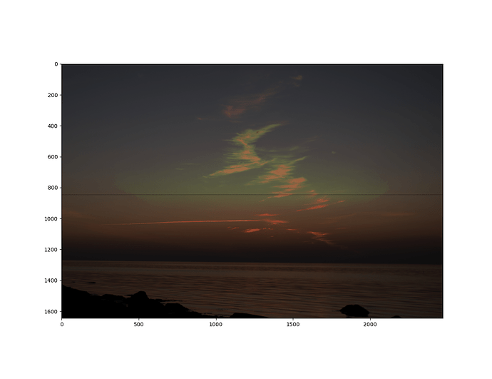
And as promised the same test but for @Iain and @hannoschwalm method!

  1. There is strong enforcement of color bleeding (uniform per patch even?) that sometimes works and sometimes causes artifacts. The artifact is visible on the same image as I used on my previous post but I graphed a line slightly lower down as the artifact is more visible there. This causes the green channel to be too high for large portions of this image resulting in the green tint.
  2. The gradient propagation seems pretty good otherwise, kind of what I had expected. (Best tested by bracketed exposure and the same kind of graph difference per pixel heat map).
  3. Unclipped channels are changed for this method as well, especially at the border of clipping for one of the channels.
  4. I think border handling is probably the weakest point of this method right now. That is where I can easily spot artifacts that should be avoidable. I think that enforcing, at least, first-order smoothness could come a long way in solving that issue!

It’s interesting to compare them, I have a harder time figuring out what happens with this one and the artifacts are different.

6 Likes

This is a particularly difficult image for our method.

Firstly, because the colour channels are not well correlated in the sky. We assume the clipped area is one colour, and the relationships between the channels are not changing. Changes in colour over the clipped area mean it works on one side of the clipped region but not the other. This is why you can see the boundary quite clearly in some places.

Secondly, we assume most detail is in the minimum of RGB, which it isn’t for this image. The clouds are just about invisible in the blue channel.

1 Like

This is a particularly interesting detail :slight_smile: For sure we don’t replace unclipped bayer data but always increase data for a photosite. The different demosaicers take this data and propagate it into the surrounding pixels too - this depends on the chosen demosaicer of course. Yes - we have to improve this part.

I don’t know if i understand fully. (With borders you probably mean “border of a clipped area”) I am not sure if smoothing is the right choice here.

Forgot about the demosaicer yesterday! Interesting how one channel is able to make another overshoot a lot!

I only meant that the function should be continuous at the border of the clipped regions. No smoothing required :slight_smile: That probably means that the uniform color assumptions have to be relaxed a little bit for a case like this. F.ex we could assume the color to be uniform locally, the size/strength of that patch could be a user variable if there is no logical constant.

Why did you pick the minimum? The largest non-clipped channel will have a higher SNR and my guess is that it might correlate better with the clipped channel just by “proximity”. Another problem with doing a hard pick on which gradient to use is that they might swap places (as in the graph for the Guided Laplacian method). Question, are there any downsides to using a weighted average or similar to pick the used gradient. The middle channel could be used but still smoothly disregarded when it approaches clipping levels.

Initially because I was extrapolating data into regions where all channels are clipped.
This is currently not in the Darktable implementation.

Using the largest non-clipped channel creats problems at the boundary between only one clipped channel an two clipped channels.

Regarding alternatives like a weighted average, I have tried a weighted average, but could not get it to work. I can’t remember why.

One thing I have done previously is to sort R,G and B values creating images for minimum, median and maximum.

Then recover the clipped regions of each of those. This allows me to average all RGB channels without worrying about including clipped pixels

1 Like


here’s the vkdt render. seems the white clipping threshold is set very “conservatively”, i needed to lower it a fair bit (see slider) to get rid of blown magenta. highlight reconstruction 1.287ms on 2080Ti.

2 Likes

That’s weird, the actual clipping level when I read it out is 1.021 +/- a tiny bit of noise for both the red and the green channel… Maybe you get the magenta cast for the same reason as in Guided Laplacians, not pushing the clipped channel up enough. Are you also transferring linear gradients 1:1?

Whatever gradients massaging you do is an iterative process. Just one iteration will not do it.

I have installed your branch, and rebuilt the build directory, but I don’t see the feathering parameters that are in the puffin picture. I have only the clipping threshold and noise parameters. Has the UI changed or is something wrong with my build?

Yes, I removed the feathering params when I changed the guiding strategy because it made them irrelevant.

1 Like

Took the time to experiment a bit on the topic. I was especially interested in why both Guided Laplacians and the vkdt implementation showed signs of a magenta cast even for smoothly varying regions where only the green channel was clipped.

My hypothesis is that they both transfer the linear gradient from the lower unclipped channel to the higher clipped channel without correcting for the magnitude of the signal. I made a simple example using Poisson image reconstruction in one dimension to show the effect. I assume constant color and only an exposure change, more on that later:

The linear gradient transfer is correctly showing the same shape as the lower channel but it is much lower than the actual signal it is supposed to reconstruct. Transfering the logarithmic gradient instead reconstructs the exact same signal as the ground truth when there is no noise. The same result but with small deviations is shown in the case of added uncorrelated noise.

Assume that the high clipped channel is the green channel. Linear gradient transfer would in that case lead to increasing amounts of magenta cast towards the middle of the clipped region. Logarithmic gradient transfer would return an almost perfect result with no color cast.

Why is this the case?
Let us assume that our color is constant within the clipping region. I.e. The RGB values all follow the same exposure function but with a different relation factor or the RGB-ratio is constant.
So, given an exposure function:

Exposure = f(x) \text{ or } f(i, j)

Then our RGB values will be that function times a factor plus uncorrelated noise

R = a \cdot f(x) + n_R \\ G = b \cdot f(x) + n_G \\ B = c \cdot f(x) + n_B \\

It becomes more interesting when we explore the gradient (lets assume there is no noise for now)

\frac{d R}{d x} = a \frac{d}{d x} f(x) \\ \frac{d G}{d x} = b \frac{d}{d x} f(x) \\ \frac{d B}{d x} = c \frac{d}{d x} f(x) \\

So if green is clipped and we want to transfer the gradient, then we can’t do

\frac{d G}{d x} = \frac{d R}{d x}

As those aren’t equal to each other. We could however do

\frac{d G}{d x} = \frac{b}{a}\frac{d R}{d x} = \frac{b}{a} a \frac{d}{d x} f(x) = b \frac{d}{d x} f(x)

But b is not known and would need to be estimated or solved for in some way. There is a special case where a = b = c and that is for whenever the color happens to be white. Thus the usual need to white balance the image before highlight reconstruction (or demosaic for that matter).

An alternative approach, as already hinted about above, is to first take the logarithm (again lets just ignore noise for now)

log(R) = log(a) + log(f(x)) \\ log(G) = log(b) + log(f(x)) \\ log(B) = log(c) + log(f(x)) \\

and then differentiate. Rember that constants such as log(a) have a slope of zero.

\frac{d}{d x} log(R) = \frac{d}{d x} log(f(x)) \\ \frac{d}{d x} log(G) = \frac{d}{d x} log(f(x)) \\ \frac{d}{d x} log(B) = \frac{d}{d x} log(f(x)) \\

All channels now have the same gradient! Which means that they can now be dropped and replaced without any need of white balancing or adjusting for colors (a, b, c differences). And it does indeed work as shown in the presented graph!

Note that low SNR close to zero will yield extremely large gradients, there probably would be a need for some sort of noise floor or noise reduction if this is to be used for real in a highlights reconstruction method.

Anyway, hope people find this little observation interesting.

PS
Poisson image editing as an approach to highlights reconstruction is another interesting topic to dive deeper into in a later post. It opens up for clone tool like transfer of gradients from one part of an image to another as well as placing “color seeds” to force a specific color if the only-exposure-changes-locally assumption fails. I can recommend this simple guide by Eric Arnebäck for anyone who wants to get familiar with the method:
https://erkaman.github.io/posts/poisson_blending.html
The downside is that you need to solve a potentially pretty large matrix inverse which probably is to slow for darktable. That said, there are iterative methods and approximisations that could trade accuracy vs speed.
DS

7 Likes

I’ll need to read through that more carefully later, but the curves you have above (noisy gaussians?) are actually much better behaved than clipped images. I’ve been testing almost exactly that myself. Local gradients are fine in certain places, but when surrounding objects are involved, the multipliers can become quite unstable.

Edit: I’ve also done tests previously with poisson editing on raws - maybe just my machine, but it was painfully slow at usual raw dimensions.

Fun that you have tried out using Poisson editing on raws! Did you work with logarithmic or linear gradients? I’m not at all surprised if it was slow, especially if you solved the full dense matrix and not the sparse version! Even a sparse exact solution is probably very slow so I think we would need either iterative or approximation methods to actually run in darktable. I think an exact Poisson method would be extremely interesting though as a way to get a baseline for approximations.

And yeah, I only showed a graph for when the assumption holds, that’s why I made a synthetic example :wink:
The only valid option I can think about atm for when the assumption doesn’t hold is to add manual tools to direct and override the solution when needed. Seeds, overrides, cloning, etc are all possible tools to fix issues like that.

On performance of Poisson editing, I note that it can be implemented with Fourier solvers, apparently with performance advantages. See http://www.iro.umontreal.ca/~mignotte/IFT6150/Articles/FourierPoissonEditing.pdf .

I don’t know if darktable uses Fourier.

A general discussion of Poisson editing is at Seamless photomontage. Since writing that, ImageMagick has incorporated “seamless-blend” and “saliency-blend” compose methods.

And that’s why it’s not what we are doing. The guided laplacian is not a direct transfer of the laplacian. It’s guided, precisely.

The guided filter is based on a local (piece-wise) model, which is a straightforward linear fitting: Filtered = a × Image + b. a and b are set by comparing a mask with the original image, such that a = \frac{cov(mask, Image)}{var(Image) + \epsilon} and b = mean(mask) - a × mean(Image). You see that \epsilon is a user param that effectively reduces the proportional part when > 0 to increase the constant part and therefore smoothen oscillations, which is where the surface blur comes from.

Laplacians are not first order gradients, but \Delta = \dfrac{d^2x}{dx^2} + \dfrac{d^2y}{dy^2}. This models the oscillations around the local average and is invariant in exposure, unlike the first-order gradient. This is what we transfer, and this is what is output by the high-frequency layer of the wavelets decomposition when you choose a cardinal B-spline wavelet (± some scaling error). In the wavelets scaling, the average magnitude of the signal will be held by the low-frequency layer).

What I do in here is detect the channel that is the best guiding candidate, such that channel = arg \,max\,(var(\Delta_{R, G, B})). This will be our guide and our best estimate of the valid signal since it has the highest variance.

With this, I model the damaged channels against this guide with a linear fit that is a bit modified compared to the guided filter (which is meant as a surface blur): Reconstructed = a × guide + b, where a = \dfrac{cov(guide, RGB)}{var(guide)}, and b = mean(RGB) - a × mean(guide). So a will ensure the oscillations taken from the guide are properly scaled before applying them on damaged channels, and b will degrade the solution to a constant average color if no satisfying correlation was found.

Rewritten as a Poisson PDE, this yields: \Delta U_{damaged} = a \Delta U_{valid} + b.

Also, we reconstruct in a pyramidal way, coarse to fine. So each scale reconstruction is added on top of the previous.

As you see, the laplacians are already rescaled. This makes me wonder if your log trick is not just a convenient ad-hoc gain that indeed fixes the problem here but may degrade things elsewhere. I don’t see what the meaning of the gradient of the log is.

3 Likes

Out of curiosity, I tried the method:

Laplacian of log RGB:

Laplacian of RGB:

Original:

Upon close inspection, the log methods slightly darkens and shifts to orange, which indeed means more green is added. But then, it still doesn’t fix magenta.

No further filmic desat/reconstruction was applied.

2 Likes

Also, on second thought, the effect of a log is to dampen large variations. It will make specular highlights and light sources closer in magnitude to reflective objects. It means there is an higher chance for reflective colors to get inpainted into speculars or light sources, which is generally wrong.

This plus the possible numerical instabilities of the log, the extra computational cost of exp/log and the very minor difference it makes, I’m not sure it’s worth it.

A mixture, but that was not in the context of highlight reconstruction (stuff like gradient blending or contrast enhancement). I used g’mic for most of that, which I believe uses libfft for inverse laplacian. Boundaries are tricky to handle.

It’s pretty fast on common desktop resolutions. I’ve also used laplacian matting C programs, but I wouldn’t bother on a raw. It takes minutes even with a small file. No surprise, given sparse matrix with dimension NxN (where N is the total number of image pixels!)

Part of that looks like linear regression, is that what you mean by linear fit?

Edit: no need to answer that, it must be indeed. Just happens to be what I was working on too…

1 Like