help: Can I get the binarized edges?

I would really appreciate it if I could borrow the forum wisdom.

First, I have a colorful picture which has smooth blurred edges. (Below “now”).
I would like to convert all edges binarizing. (Below “want”)
Can I achieve this by G’MIC?

(I tried Posterise. It is ideal action to make binarized edges, but It’s has no option to keep colors what I want. so I stucked)
(WHY: I would like to make the material ID map from my texture map, so I need binarized edges.)

colorregions:
   # Test image to emulate your input texture map: Mostly solid regions with
   # slightly fuzzy borders.
   
   -input 128,128,1,3
   -turbulence 30,4,5

   # First argument to -autoindex sets the number of solid colors, here 4.
   # You would know before hand how many dominant colors there are in your
   # texture.
   
   -autoindex. 4,0,1
   -name. testimage

   # Finish the test image by fuzzing the borders probably more than
   # what is typical for your case.
   
   -blur. 2

   # Here's where we attempt to reconstruct sharp borders.
   # Your solution starts here.

   # Determines what are the most dominant colors in the texture.
   # You know this. So, instead of '4', choose the actual count. For
   # example, your test case has five dominant colors

   +colormap[testimage] 4,1

   # Name is just to document image roles. Not fundamental to the solution.
   -name. palette

   # Make an index map
   +index[testimage] [palette],0
   -name. indexmap

   # Map indexed regions to palette colors.
   +map[indexmap] [palette],3

The first part of this script is just to make an arbitrary test image emulating your circumstances. colormap finds the x dominant colors; you choose x based on your texture design. colormap produces a palette of these dominant colors. index thresholds your fuzzy-border image so that pixels align with one dominant color or another. If borders are really, really fuzzy, as in this example, you may not recover exactly the location of the original border. You may not care about
this as you are dealing with not very fuzzy borders. Finally map reintroduces the original dominant colors — and I think you are home free.

Give this a whirl on the Wurlitzer and see if it plays. Let us know how this turns out.

3 Likes

As I was writing this, I was thinking this was a tad too over-engineered. Your shorter, faster solution
is just:

…
   -autoindex[myfuzzypicture] $countofdominantcolors,0,1
…

Have fun.
G.

I wonder if there is an algorithm that exist which can get the number of dominant colors or estimate the number of dominant color. This with conjunction with autoindex can be performed on multiple pictures at once when there are different numbers of dominant colors.

I looked at google. Zero results.

Also, yes autoindex is the most reasonable solution here.

Perhaps something with distance threshold to determine the likely number of dominant color? If the color distance is close to another color, they’re grouped as one. I wish I knew how to do that though.

There is.
From the Ancien Régimes
G’MIC Color Mapping

In particular, the K-T Means algorithm, implemented in colormap.

One of the many old tutorials needing portage to modern times…

Could you put the full original image to process so we can try to play with it?

I may have something here:

round +colormap 0,,0 +index[-2] [-1],0,0 +area. 0,0 remove[1]


Next step is to find the most common areas i.e all colored areas with size greater than the average size, and to use that to find the most common color within colormap 0,,0. I just haven’t figured out this yet. But, certainly, I believe this is feasible.

I don’t think average works well.

FInal solution attempt:

round +colormap 0,,0 +index[-2] [-1],0,0 +area. 0,0 gt. {ia/2} *.. . negate. -.. . rm. colormap. 0,,1 crop. 1,100% map. .. rm.. index.. .,0,1 rm.

image
image
image

The problem with autoindex is that it may put undesired colors at the transitions, just because one of the plain color somewhere else is close enough.
Typically :

foo :

  # Generate example image.
  srand 0 100,100 plasma 1,1 b 3,0 quantize 8,0 n 0,100
  map lines smooth 30,0,1

  # Quantize and save outputs.
  +autoindex 8
  o[0] "input.png"
  o[1] "quantized.png"

  # Render montage.
  +z 7,60,0,43,91,0
  r2dy 300,1
  to[0] Input
  to[1] "Quantized (8 colors)"
  to[2] "Input (zoom)"
  to[3] "Quantized (zoom)"
  frame 1,1,0 frame 3,3,255 a x

Here you see that between the dark blue and the green, autoindex has inserted pixels with the darker green that is a color present elsewhere in the image.
Not good.

At this point, I’m not sure what would be the best approach for this particular image. I put it here, because it seems challenging enough for me :slight_smile:

input

Out of curiosity, I’ve tested the online Adobe service to convert png to svg, and this leaves clear artefacts on this particular image:

input_adobe_express

Hmm, regarding my earlier approach, can be even improved further by having minimum distance per area as a image, so one can have a slight more control in which areas is more acceptable. However, it’s good enough for most cases.

EDIT: Because of rounding, it appears to have issue with some color space. I don’t see a way out of that if blur is used. I guess it’s up to users to multiply the value of images in some cases. There’s also the limitation of small blurry areas are seen as an area, but manually easily fixable. Finally, the more color with separate region, the worse this filter can perform, but I haven’t hit that issue yet as it still works for 40+ color.

Pseudo-code:

  1. Reduce color mode.
  2. decrease size
  3. increase size

'gmic' ~/try1.png r 100,100 r 400,400 -output try1-out.png
try1try1-out

I wanted to add a color indexing step in #1 but couldn’t get that to work.

Yes. I think the pathological condition arises when some colors are co linear in the RGB color space. One of my colors is a complement of another and a third is nearly gray: they form a line passing through the center of the color cube. The pathology doesn’t require passing through the center of the color cube, just that (some) chosen colors are co linear with others so that there are midway colors on the lines connecting complements. Then, even with the slightest blur, there will be transition pixels on the border between complements that would be midway colors, even if pixels of such colors were not present in the original (unblurred) image.

This is not a problem that just sits with autoindex; that command is just a wrapper around colormap and index; the heart of the matter lies with a particular color geometry. Even my original proposal would be susceptible to this pathology. What this means in simpler terms is that there will be some color combinations that will not resolve well.

I have to wonder if there is an algorithm in which sections of color joins other sections of color using the farthest distance away from blurred edge. The farthest color is used as patch color. As soon as it meets the skeleton of blurred edge, it is considered as one patch. Would be perfect for this. I noticed that even my solution has the problem @grosgood and @David_Tschumperle observed though albit to a less extent. Honestly, this seem like research paper material.

I tested my code on David’s image, it didn’t work out. Still just as bad.

EDIT:

The following code allows me to detect blurred edges

rep_norm_difference:
skip ${1=3}

number_of_images={$!}

radius={r=int(abs($1));!(r&1)?++r;r;}

{vector(#2,$radius)},1,2,"begin(
  const center_pos=w>>1;
 );
 [x-center_pos,y-center_pos];
 "

resize. 1,{whd},1,100%,-1 ({h})
append[-2,-1] y

eval da_remove(#-1,da_size(#-1)>>1);da_freeze(#-1);

repeat $number_of_images {
  
  {w#0},{h#0},1,1,"
   const radius=$radius;
   const number_of_offset=radius*radius-1;
   const offset_image_position=$number_of_images;
   distance=0;
   current_color=I#0;
   repeat(number_of_offset,ind_pos,
    distance+=norm(current_color-J(#0,I[#offset_image_position,ind_pos],0,3));
   );
   distance;
   "
   
  remove[0]
}

remove[0]

Results here:

So, in conjunction with inpaint,label, and shape_average, and the technique I used earlier, I would consider this solved.

Also, modifying the above code seem to reveal a presence of skeleton:

image

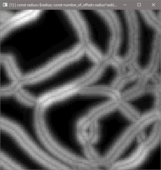
If one can get that skeleton and label the inside areas, then this thread can be solved.

So, I think it is definitely possible. Computationally intensive though.

Exactly, that’s why a better solution should involve some kind of spatial analysis/filtering of the image, not only color transformations.

A promising approach is to iterate a shock filter (implemented by the native sharpen command in G’MIC) until the change from one iteration to another becomes low enough.
This is still not perfect, but it leaves few artifacts on my difficult image, compared to all the other methods I’ve tested.
This:

foo :
  input.png
  do
    +sharpen 1,1
    -.. . norm.. diff={-2,iM} rm..
    w. 500,500
  while $diff>1

Before/after:
before_after

And I didn’t even quantize the output image :slight_smile:

2 Likes

I have been following this and @David_Tschumperle your latest foray is the direction I would have gone. Perhaps, you may try doing a hybrid between per channel and norm delta.

1 Like

With the same code I think, but I’ll just share the current code in spoiler.

rep_norm_difference code
rep_norm_difference:
skip ${1=3}

number_of_images={$!}

radius={r=int(abs($1));!(r&1)?++r;r;}

{vector(#2,$radius)},1,2,"begin(
  const center_pos=w>>1;
 );
 [x-center_pos,y-center_pos];
 "

resize. 1,{whd},1,100%,-1 ({h})
append[-2,-1] y

eval da_remove(#-1,da_size(#-1)>>1);da_freeze(#-1);

repeat $number_of_images {
  
  {w#0},{h#0},1,1,"
   const radius=$radius;
   const number_of_offset=radius*radius-1;
   const offset_image_position=$number_of_images;
   distance=0;
   current_color=I#0;
   found_offset=0;
   repeat(number_of_offset,ind_pos,
    v=norm(current_color-J(#0,I[#offset_image_position,ind_pos],0,3));
    distance+=v;
   );
   distance;
   "
   
  remove[0]
}

remove[0]

I was able to do this:

$ +rep_norm_difference , normalize_local. 5,5,10%,2% gt. {ia} skeleton. 0 negate. label_fg. 0,0 +blend shapemedian0 +colormap. 0,,1 crop. 1,100% +store[0] image index[0] [-1],0,1 eq[1] 0 image[2] [0],0,0,0,0,1,[1] rm. $image rv[0,-1] rm.

If only skeleton was faster. Also, still some issues with my approach. See closeup:

image

EDIT: I believe I know my solution, in the edge image, when pixel at edge, search around non-pixel edge, and find color that closest match to original image using found colors

Promising. A few curios from the Ye Olde Curio Shoppe.

Clown face:
clown

Clown face, slightly defaced (-blur 1):
clown_blur

Shock filter, slightly modified for metrics:

shock :
  0
  -name. diffhist
  -move[diffhist] 0
  -do
    +sharpen. 1,1
    -sub.. .
    -norm..
    diff={-2,iM}
    -remove..
    -eval {da_push(#$diffhist,$diff)}
  -while $diff>1
  -eval. {da_freeze(#$diffhist)}
  -display_graph[diffhist] 1024,400,1,0,0,0,0,0,"Iterations","Diff"

The normalized difference exhibits a directional bias:
clown_diff
This snapshot is from the first iteration around, just before the -remove.. step.

Display graph of convergence:

result:
clown_s

Pretty good, but where slight blurring remains is along a horizontal direction. I think I perceive a similar effect in @David_Tschumperle results: failure there, also slight, seems to exhibit horizontal preference. Methinks that is why convergence is longer than it could be: this approach is being blind-sided by horizontally oriented blurring. Such does not “dissolve” as rapidly as blurring in other orientations.

Why wouldn’t -sharpen exhibit pan-directional behavior? Time to answer my own question…

1 Like

Hmm, couldn’t one just use a stacked rotated image, then check which is closest match to blurred image to dodge the horizontal artifact?

Another try, another hope to get it better… :slight_smile:

The idea here is :

  • First, detect the transition pixels, simply with a threshold on the area of constant regions.
  • Second, for each pixel to reconstruct (transition pixel), count the different colors in a NxN neighborhood. Keep the two main colors and determine what is the closest one to the central pixel.

Doing this, you get a reasonnable outcome, similar to what shockfilters do, but in a single iteration, and without all the small color variations (because we basically do local quantization in 2 colors).

Here is the code:

foo :
  +label 0,1 area. 0,1 ge. 3 negate. # Determine transisition points
  f[0] "
    begin(
      const boundary = 1;
      const N = 5;
      const N2 = int(N/2);
    );

    i(#-1)?(
      # Count color occurences in a NxN neighborhood.
      RGBs = vector(#3*N^2);
      occs = vector(#N^2);
      nb = 0; # Number of different colors counted
      repeat (N,q,
        repeat (N,p,
          RGB = I(x + p - N2,y + q - N2);
          found = 0;
          repeat (nb,k,rgb = RGBs[3*k,3]; rgb==RGB?(found = 1; break()));
          found?++occs[k]:(++occs[nb]; copy(RGBs[3*nb],RGB); ++nb);
        );
      );

      # Find two closest colors.
      ind0 = argmax(occs); RGB0 = RGBs[3*ind0,3]; occ0 = occs[ind0]; occs[ind0] = -1;
      nb>1?(
       ind1 = argmax(occs); RGB1 = RGBs[3*ind1,3]; occ1 = occs[ind1]
      ):(
        ind1 = ind0; RGB1 = RGB0; occ1 = occ0;
      );

      occ0 - occ1<=1?(
        RGB = I;
        norm(RGB - RGB0)<norm(RGB - RGB1)?RGB0:RGB1
      ):RGB0
    ):I"
  rm.

And the result, on the challenging image:

$ gmic input.png foo

I think the next step would be to count the colors, not in a square neighborhood centered at each pixel, but on an oriented segment whose direction is given by the main eigenvector of the structure tensor.
Will try later if I have time to do so :slight_smile:

PS: And honestly, it’s too good to be able to do that with so few lines of code. G’MIC rocks! :slight_smile:

1 Like

See ImageMagick – Command-line Options

magick davidblobs.png -paint 1 d.png

d

dLgt

1 Like

@snigbo, interesting, what’s the algorithm used for -paint?