New Sigmoid Scene to Display mapping

[anon41087856]

@jandren

It should at least be similar because they are not drastically different in the results from each other. I’m currently trying to reverse engineer the filmic polynomials to have a better 1D baseline/comparison, will post the results when they are ready.

Don’t.

From [1] : (I copy-paste here because MathJax doesn’t load anywore on my website, so LaTeX doesn’t render for now).

The software then translates the parameters into 2D nodes that will be fed to the interpolation algorithm:

• grey = \{\text{G}_{l} ; \text{G}_{d} \} \\= \{ \frac{- \text{black}_{EV}}{ \text{DR}} ; 0.18^{1/\gamma} \}
• black = \{ 0 ; 0 \}
• white = \{ 1 ; 1 \}
• latitude, bottom = \{ \text{T}_{l} ; \text{T}_{d} \} \\= \{ \text{G}_{l} × \left(1 – \frac{\text{latitude}}{ \text{DR}} \right) ; \text{C} × \left(\text{T}_{l} – \text{G}_{l}\right) + \text{G}_{d} \}
• latitude, top = \{ \text{S}_{l} ; \text{S}_{d} \} \\= \{ \text{G}_{l} + \frac{\text{L}}{\text{DR}} × (1 – \text{G}_{l}) ; \text{C} × (\text{S}_{l} – \text{G}_{l}) + \text{G}_{d} \}

\begin{cases} P_1′(x) &= \text{C}\\ P_1(\text{T}_{l}) &= \text{T}_{d}\\ P_0(0) &= 0\\ P_0′(0) &= 0\\ P_0(\text{T}_{l}) &= \text{T}_{d}\\ P_0′(\text{T}_{l}) &=P_1′(\text{T}_{l}) \\ P_0”(\text{T}_{l}) &=P_1”(\text{T}_{l}) \\ P_2(1) &= 1 \\ P_2′(1) &= 0 \\ P_2(\text{S}_{l}) &= \text{S}_{d} \\ P_2′(\text{S}_{l}) &= P_1′(\text{S}_{l}) \\ P_2”(\text{S}_{l}) &= P_1”(\text{S}_{l}) \\ \end{cases}

Each polynom needs to satisfy 5 conditions, therefore we need 4th order polynoms. Let us parametrize such functions \forall \{x, a, b, c, d, e, f, g, h, i, j, k, l\} \in \mathbb{R}^{13} :

\begin{cases} P_0(x) &= a x^4 + b x^3 + c x^2 + d x + e\\ P_1(x) &= f x + g\\ P_2(x) &= h x^4 + i x^3 + j x^2 + k x + l\\ \end{cases} \\ \Rightarrow \begin{cases} P_0′(x) &= 4 a x^3 + 3 b x^2 + 2 c x + d \\ P_1′(x) &= f \\ P_2′(x) &= 4 h x^3 + 3 i x^2 + 2 j x + k \\ \end{cases} \\ \Rightarrow \begin{cases} P_0”(x) &= 12 a x^2 + 6 b x + 2 c \\ P_1”(x) &= 0 \\ P_2”(x) &= 12 h x^4 + 6 i x + 2 j \\ \end{cases}

This can be split into 3 linear sub-systems for faster resolution, the last two being solvable in parallel :

P_1 : \begin{bmatrix} 1 & 0 \\ \text{T}_l & 1\\ \end{bmatrix} \cdot \begin{bmatrix}f\\g\\\end{bmatrix} = \begin{bmatrix} \text{C}\\ \text{T}_d\\ \end{bmatrix}

P_0 : \begin{bmatrix} 0 & 0 & 0 & 0 & 1\\ 0 & 0 & 0 & 1 & 0\\ \text{T}_l^4 & \text{T}_l^3 & \text{T}_l^2 & \text{T}_l & 1\\ 4 \text{T}_l^3 & 3 \text{T}_l^2 & 2 \text{T}_l & 1 & 0\\ 12 \text{T}_l^2 & 6 \text{T}_l & 2 & 0 & 0\\ \end{bmatrix} \cdot \begin{bmatrix}a\\b\\c\\d\\e\\ \end{bmatrix} = \begin{bmatrix} 0\\ 0\\ \text{T}_d\\ f\\ 0\\ \end{bmatrix}

P_2 : \begin{bmatrix} 1 & 1 & 1 & 1 & 1\\ 4 & 3 & 2 & 1 & 0 \\ \text{S}_l^4 & \text{S}_l^4 & \text{S}_l^2 & \text{S}_l & 1 \\ 4 \text{S}_l^3 & 3 \text{S}_l^2 & 2 \text{S}_l & 1 & 0\\ 12 \text{S}_l^2 & 6 \text{S}_l & 2 & 0 & 0\\ \end{bmatrix} \cdot \begin{bmatrix}h\\i\\j\\k\\l\end{bmatrix} = \begin{bmatrix} 1\\ 0\\ \text{S}_d\\ f\\ 0\end{bmatrix}

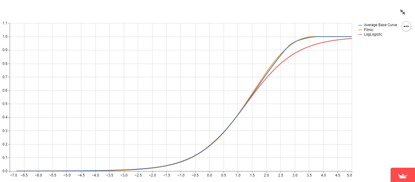
Solving the polynomial coefficients for the input nodes can be achieved through a gaussian elimination, then, in a vectorized SIMD/SSE setup of 4 single precision floats using Fused Multiply-Add, a fast evaluation of S(y) should be possible such that:

S(y) = \left[ \begin{bmatrix} e \\ g \\ l\\ 0\\\end{bmatrix}+ y \cdot \left(\begin{bmatrix} d \\ f \\ k\\ 0\\\end{bmatrix} + y \cdot \left(\begin{bmatrix} c \\ 0 \\ j\\ 0\\\end{bmatrix} + y \cdot \left(\begin{bmatrix} b \\ 0 \\ i \\ 0\\\end{bmatrix} + y \cdot \begin{bmatrix} a \\ 0 \\ h \\ 0\\\end{bmatrix} \right) \right) \right) \right] \cdot \begin{bmatrix} (y < \text{T}_l)\\ (\text{T}_l \leq y \leq \text{S}_l)\\ (y > \text{S}_l)\\ 0\\ \end{bmatrix}^T the last matrix being an boolean mask where lines are set to 1 where the condition is met, or 0 otherwise.

---

Just note that the curve is applied in log normalized space, so y = \dfrac{\log_2 \left(\frac{x}{\text{grey}}\right) – \text{black}_{EV}}{\text{white}_{EV} – \text{black}_{EV}}

[anon41087856]

Aaand I just found the Python prototype…

%matplotlib notebook
import numpy as np
import matplotlib
matplotlib.rcParams['pdf.fonttype']=42
matplotlib.rcParams['ps.fonttype']=42
import matplotlib.pyplot as plt
from ipywidgets import interact
plt.style.use('bmh')

# define the curve via these control vertices here:
x=np.array([0.3,0.45,0.80,1.00])
y=np.array([0.0,0.62,0.14,0.97])

m=np.array([0.0,0.0,0.0,0.0,0.0])
d=np.array([0.0,0.0,0.0,0.0,0.0])

def fma(a, b, c):
    # fake FMA just for the logic of it
    return a * b + c


def filmic_spline_draw(x, coeffs, toe, shoulder):
    # coeffs = [a, b, c, d, e, f, g, h, i, j, k, l]
    # s.t. :
    # P0 = ax⁴ + bx³ + cx² + dx + e
    # P1 = fx + g
    # P2 = hx⁴ + ix³ + jx² + kx + l
    # latitude = [toe ; shoulder] < dynamic range
    # See https://bit.ly/2IXfLnQ
    
    # build the value masking row vector
    part0 = x < toe
    part2 = x > shoulder
    part1 = part0 == part2 # where part0 == part2 == False, toe < x < shoulder
    mask = np.array([part0, part1, part2])
    
    # make x a 2D row vector
    x = x[np.newaxis, :]
    
    # unpack coeffs
    a = coeffs[0]
    b = coeffs[1]
    c = coeffs[2]
    d = coeffs[3]
    e = coeffs[4]
    f = coeffs[5]
    g = coeffs[6]
    h = coeffs[7]
    i = coeffs[8]
    j = coeffs[9]
    k = coeffs[10]
    l = coeffs[11]
    
    # repack coeffs as column vectors
    M1 = np.array([[e, g, l]]).transpose()  # const
    M2 = np.array([[d, f, k]]).transpose()  # factors of x
    M3 = np.array([[c, 0, j]]).transpose() # factors of x²
    M4 = np.array([[b, 0., i]]).transpose() # factors of x³
    M5 = np.array([[a, 0., h]]).transpose() # factors of x⁴
    
    # evaluate the 3 parts of the curve
    y = fma(x, fma(x, (fma(x, fma(x, M5, M4), M3)), M2), M1)
    
    # apply masks and sum
    return (y * mask).sum(axis=0)


def filmic_desaturation_draw(x, coeffs, toe, shoulder):
    # coeffs = [a, b, c, d, e, f, g, h, i, j, k, l]
    # s.t. :
    # P0 = ax⁴ + bx³ + cx² + dx + e
    # P1 = fx + g
    # P2 = hx⁴ + ix³ + jx² + kx + l
    # latitude = [toe ; shoulder] < dynamic range
    # See https://bit.ly/2IXfLnQ
    
    # build the value masking row vector
    part0 = x < toe
    part2 = x > shoulder
    part1 = part0 == part2 # where part0 == part2 == False, toe < x < shoulder
    mask = np.array([part0, part1, part2])
    
    # make x a 2D row vector
    x = x[np.newaxis, :]
    
    # unpack coeffs
    a = coeffs[0]
    b = coeffs[1]
    c = coeffs[2]
    d = coeffs[3]
    e = coeffs[4]
    f = coeffs[5]
    g = coeffs[6]
    h = coeffs[7]
    i = coeffs[8]
    j = coeffs[9]
    k = coeffs[10]
    l = coeffs[11]
    
    # repack coeffs as column vectors
    M3 = np.array([[c, 0, j]]).transpose() # factors of x²
    M4 = np.array([[b, 0., i]]).transpose() # factors of x³
    M5 = np.array([[a, 0., h]]).transpose() # factors of x⁴
    
    # evaluate the 3 parts of the curve
    y = 2 * fma(x, 3 * fma(x, 2 * M5, M4), M3)
    
    # apply masks and sum
    return np.abs((y * mask).sum(axis=0)) / 8.


def filmic_spline_solve(T_l, T_d, S_l, S_d):
    
    # Contrast/slope of the latitude
    C = (S_d - T_d) / (S_l - T_l)
    
    # Get params of the linear part : P1 = fx + g
    M1 = np.array([[1.  ,  0.], 
                   [T_l ,  1.]])
    y1 = np.array([C, T_d])
    P1 = np.linalg.solve(M1, y1)
    
    f = P1[0]
    g = P1[1]
    
    # Get params of the cubic toe P0 = ax⁴ + bx³ + cx² + dx + e
    M0 = np.array([[0.           , 0.          , 0.       , 0. , 1.],
                   [0.           , 0.          , 0.       , 1. , 0.],
                   [T_l**4       , T_l**3      , T_l**2   , 1. , 0.],
                   [4. * T_l**3  , 3. * T_l**2 , 2. * T_l , 1. , 0.],
                   [12. * T_l**2 , 6. * T_l    , 2.       , 0. , 0.]])
    y0 = np.array([0., 0., T_d, f, 0.])  
    P0 = np.linalg.solve(M0, y0)
    
    a = P0[0]
    b = P0[1]
    c = P0[2]
    d = P0[3]
    e = P0[4]
    
    # Get params of the cubic shoulder P2 = hx⁴ + ix³ + jx² + kx + l
    M2 = np.array([[1.           , 1.          , 1.      , 1. ],
                   [S_l**3      , S_l**2  , S_l , 1.],
                   [3. * S_l**2 , 2. * S_l, 1. , 0.],
                   [6. * S_l    , 2.      , 0. , 0.]])
    y2 = np.array([1., S_d, f, 0.])
    P2 = np.linalg.solve(M2, y2)
    
    h = 0.
    i = P2[0]
    j = P2[1]
    k = P2[2]
    l = P2[3]
    
    # pack the params of the solution
    return [a, b, c, d, e, f, g, h, i, j, k, l]


fig, ax = plt.subplots(figsize=(5,5))
ax.set_ylim([-2.,2.])
ax.set_xlim([-2.,2.])
pos = np.linspace(0., 1., 1000) # 4 Mpix to make benchmarks meaningful
ax.axvline(x=0.0,ymin=0.0,ymax=1.0)
ax.axvline(x=1.0,ymin=0.0,ymax=1.0)
px1 = ax.axvline(x=x[1],ymin=0.0,ymax=1.0)
px2 = ax.axvline(x=x[2],ymin=0.0,ymax=1.0)
ax.axhline(y=0.0,xmin=0.0,xmax=1.0)
ax.axhline(y=1.0,xmin=0.0,xmax=1.0)
plot1 = ax.plot(pos, np.zeros(pos.shape), color='C1')[0]
plot2 = ax.plot(pos, np.zeros(pos.shape), color='C3')[0]
plot3 = ax.plot(pos, np.zeros(pos.shape), color='C5')[0]


@interact(ix1=(0.0,1.0,0.01),ix2=(0.0,1.0,0.01),iy1=(0.0,1.0,0.01),iy2=(0.0,1.0,0.01))
def test_spline(iy1=0.55, iy2=0.92, ix1=0.67, ix2=0.92):
    y[0] = 0.
    y[1] = iy1
    y[2] = iy2
    y[3] = 1.
    x[0] = 0.
    x[1] = ix1
    x[2] = ix2
    x[3] = 1.
    
    px1.set_xdata(x[1])
    px2.set_xdata(x[2])
    
    # plt.plot(pos, np.power(pos, 0)*c[0]+ pos*c[1] + pos*pos*c[2] + pos*pos*pos*c[3])
    
    setup_spline()
    plot1.set_ydata(np.array([hermite(t) for t in pos]))
    
    params = filmic_spline_solve(ix1, iy1, ix2, iy2)
    y_filmic = filmic_spline_draw(pos, params, ix1, ix2)
    plot2.set_ydata(y_filmic)
    
    y_desat = filmic_desaturation_draw(pos, params, ix1, ix2)
    plot3.set_ydata(y_desat)
    
    ax.legend((plot1, plot2, plot3), ["Hermite", "Filmic", "Desaturation"])
    fig.canvas.draw()

# test_spline(0.0, 0.2, 0.8, 1.0)

[jandren (Jakob Andrén)]

Thank you!

That will take me closer to comparing the two and get a proper understanding of how filmic behaves. I will still need to do some digging in the c code though as I want to expose the user sliders and make a comparison that way. I’m a sucker for graphs so making a direct 1D comparison makes a lot of sense to me on the way to really taste the secret sauce!

[PhotoPhysicsGuy (Bob)]

Not sure if this should be a separate post, go into the OKlab thread, or should live here:

There is a new blogpost by Björn Ottosson @bottosson https://bottosson.github.io/posts/gamutclipping/ which I find once again, extremely inductive, easy to read and well presented. @jandren I think that’s well worth a read for you too.

While dealing with specific implementations of two algorithms for handling of gamut clipping, there is certainly valuable insights into topics that will frequently come up in the context of (but not limited to) Scene-to-Display mapping.

And while not explicitly designed with HDR in mind, techniques and approaches should be implicitly similar.

[age]

@jandren

I do really like the way especially the highlights looks, with a smooth rollover to a desaturated white.

Some tests
The test image is a hdr pattern , it goes from 900 nits to 4000 nits
test_pattern008639_01.tif (11.5 MB)

test image converted to sdr with clipping

converted to sdr with reinhard tmo on rgb channels

converted to sdr with reinhard tmo and aces desaturation

converted to sdr with darktable’s filmic and preserve chrominance

converted to sdr with darktable’s filmic , no color preservation and aces desaturation before the module

test_pattern008639_01.tif.xmp (9.8 KB)

[jandren (Jakob Andrén)]

Those are some really nice tests @age!

Just to be sure I understood you correctly, reinhard tmo is this?
https://64.github.io/tonemapping/#reinhard
i.e.
display = scene / (1 - scene)
Which basically is a subcase of the log-logistic sigmoid when the power/contrast = 1?

Because the case with aces desaturation + Reinhard curve looks really nice to me. Both hue and saturation wise! Is there anything to complain about for this one? Is there anything wrong with the hue? What would a correct hue look like in that case?

The default filmic looks similar to the ACES synthetic charts I posted with a quite aggressive desaturation. Too aggressive for my taste.

[age]

@jandren

Just to be sure I understood you correctly, reinhard tmo is this?
Tone Mapping | δelta
i.e.
display = scene / (1 - scene)
Which basically is a subcase of the log-logistic sigmoid when the power/contrast = 1?

I have used the extended reinhard tmo in the same page, where C white is 40 for this image, so I could map the max value to 1.

@jandren

Is there anything wrong with the hue? What would a correct hue look like in that case?

Well, using the ICtCp color space gives this result

For comparison Madvr that works in ictcp too, render this frame as such

[age]

@jandren

Because the case with aces desaturation + Reinhard curve looks really nice to me. Both hue and saturation wise! Is there anything to complain about for this one?

It looks good, there is a sligthly hue shift for red and blue hues but i think is really hard to spot with real photos

[jandren (Jakob Andrén)]

I have spent some time doing tests myself!
But I have been focusing on the 1D tone curve or Tone Mapping Operator, ignoring colors altogether for now. There will always be a curve for mapping scene intensities to a displayable range regardless of the employed color preservation method.

I kind of went all-in on the task and made myself an interactive tool, please try it yourself here:
https://share.streamlit.io/jandren/tone-curve-explorer

I found it super helpful to play around with the tone curves like this as it gave me a better understanding of the properties of the curves rather than the look they produce. Here are some of my observations:

The Log-Logistic Curve

• Models most of the average base curve very well with contrast=1.65, except the brightest part where it gives more room for highlights. I think the average base curve is very relevant here as a kind of meta-study of multiple camera companies, their engineers, testers, and managers.
• Always returns a slope with a single peak + smooth tails independent of contrast setting.
• Works well for any target black < target grey and target white > target grey (actual look on an HDR monitor TPD).
• Contrast < 1 will have peak contrast at luminance zero. Might seem weird at first but make sense when you study how the value curve changes with lower contrast.
• Possible improvement: Introduce a skewness parameter for shifting the peak contrast towards shadows or highlights!

The Filmic Curve

• Is not a superset, for any contrast setting, of the Log-Logistic Curve.
• Does not guarantee: slope >= 0, slope peaks = 0, or target white >= output >= target black
• White and black relative exposure seems to be defined mostly to make the spline model work.
• Every other setting is covariant with the white and black relative exposure. Contrast is for example the slope in the normalized computational [0,1] range and not related to the absolute image contrast.
• Latitude and Balance are defined as relative to the dynamic range and usually needs to be retuned if the contrast setting is changed.
• Auto hardness does not work well when, target black != 0 or when target white != 1
• The purpose of hardness, sometimes called gamma in the documentation, seems to mostly be about making the spline setup work for that particular combination of display and scene luminances.
• My general feeling is that I have 8 parameters to tune, but only a narrow tunnel of actual good/correct settings in this 8-dimensional space. I would personally say that the actual degree of freedom of the filmic curve is about two, contrast + skewness, but with manual overhead and traps. So I will not blame anyone for saying that it is hard to use!

Please share your experiences as well!

[jandren (Jakob Andrén)]

I think I variation of this chart would be interesting.
Assume middle grey = 0.1845
Let the border and the middle patch luminance be middle grey.
Let patches to the left of the middle step down one or EV per patch and step up on the right.

We would then have middle grey as the target hue to compare against. I feel like both the ICtCp and the desaturation + TMO are good when comparing patch to border, but there is defiantly a clear change in overall hue between the methods. Basically makes me wonder how the hue changes as lightness progresses from dark to bright. An not just bright to brighter

[age]

@jandren

I kind of went all-in on the task and made myself an interactive tool, please try it yourself here:
https://share.streamlit.io/jandren/tone-curve-explorer

It doesn’t works anymore, however this is my latest preset without the bakened exposure compensation ( I have the latitude set to 0.1 and middle gray at 9%)
https://discuss.pixls.us/t/new-filmic-preset-adobe-standard-tone-curve/20653/18

[jandren (Jakob Andrén)]

Hey not bad at all, and funny how well it follows the average base curve! And this was only possible to do by lowering middle grey to 0.09 or did you do that to align with a typical raw image? Do you have the actual Adobe curve available in some way? Would be fun to add it as another reference curve to the plot. And checked your topic and saw that you tested Blenders Filmic, do you have the tone curve for that as well? I tried extracting it from the code but haven’t managed as of yet. Would love to add Blenders Filmic as another reference option!

Unfortunate about the script on streamlit. Couldn’t find much info on the admin side but a reboot fixed it at least! Just check out the source and run it locally if the script on streamlit goes down again: GitHub - jandren/tone-curve-explorer: A simple streamlit app to explore the shapes of some tone curves.

[PhotoPhysicsGuy (Bob)]

@jandren

Please share your experiences as well!

Amazing. Thanks for that little toy to play with.

Log-Logistic:

• that one parameter in its simplistic glory, has its limit for me when I’d want to adjust how much of the highlights I want to push back into display range. (not solved by what toneEQ does in scene-referred)
• I like the smoothness of the curve and it’s first derivative. That seems like an inherently good idea. Certain tonality changes to fine tune contrast-appearance live in a display referred space anyway, as they are informed by the display medium characteristics.
• skewness seems a straightforward.

Filmic

• good to know it’s not a superset. Also unfortunate. I would have thought 8 parameter splines could fit a slightly more complex log-curve.
• parameter changes do all sorts of curve adjustments at once. you can’t identify a problem area and know which parameter to tweak. tweaking one parameter will change multiple aspects of the curve.
• monotonic and non-monotonic undershoots and overshoots depending on paramters chosen (basically producing artefacts)

I don’t see those things as too dramatic. For display space one could always blend between two stable filmic-curves, as long as extending the display dynamic range doesn’t break curves (at the moment it does break the curve in a weird way when you tweak the dispaly range with certain settings).

In general I think the comparison to the Average basecurve is not super relevant (but certainly interesting and a good justification for a log-logistic like curve). Why? Because I don’t think that basecurves of camera manufacturers were designed with HDR compatibility in mind.

Awesome work!

[PhotoPhysicsGuy (Bob)]

@age

For comparison Madvr that works in ictcp too, render this frame as such

Madvr has had a lot of input of people testing stuff and catching mistakes. There is at least two gigantic threads of what madshi is doing, one on doom9 and one on avsforum. I stopped reading two years ago or so. maybe it’s time for me to catch up. usually the stuff he does is quite sound.

[jandren (Jakob Andrén)]

Glad you liked it!

I’m not sure what you mean with

… adjust how much of the highlights I want to push back into display range.

Would you like control of the “punchyness” of the highlights by controlling how fast it converges to target brightness? As in what a skewness parameter would add or is it something else?

The average base curve is a central piece for me, it is too subjective to only look at images when checking how well a tone curve model performs. Making sure that I can reliably model at least the average base curve gives me a more objective metric to work against. The HDR part is best covered by adding one or several HDR “base curves” to the plot and making sure that the proposed parametric model can fulfill those as well!

So if anyone has example tone curves from HDR processed images, please share!

[PhotoPhysicsGuy (Bob)]

@jandren

Would you like control of the “punchyness” of the highlights by controlling how fast it converges to target brightness?

Yes, without affecting too much of the prior chosen curve. ‘highlight punchyness’ or ‘highlight detail’ or highlight recovery’ however you want to call it.

BUT let me be clear that I would be open to discussing whether this must be part of display mapping or not. I’d say for now yes. For compatibility with future HDR workflows though, I see that this is not an easy discussion. This also overlaps with what people use ToneEQ for.

@jandren

Making sure that I can reliably model at least the average base curve gives me a more objective metric to work against.

So a sanity check to see that a new scene-to-display curve does no weird stuff.

@jandren

The HDR part is best covered by adding one or several HDR “base curves” to the plot and making sure that the proposed parametric model can fulfill those as well!

Unless there is a way of displaying images on a HDR display with a result that is pleasing to the eye, no such curves exist, except in video land where everything is graded for a new output anyway. Aren’t there, rec.2100 ODTs for ACES? All of this prepping for HDR image workflows is a good idea that lacks the means of testing it (AFAIK, correct me if I am wrong).

[afre (Alan)]

It heavily depends on the direction industry takes. Question marks in the meantime.

[priort (Todd Prior)]

Maybe pull something from the blender world?? I think there are some curves in the blender filmic module…I have no experience with it but I have seen it demonstrated a few times??

[paperdigits (Mica)]

@priort

I think there are some curves in the blender filmic module

That is where the filmic rgb module comes from.

[afre (Alan)]

Originally, but Aurélien put a lot of work into making what it is today. @Carmelo_DrRaw has his versions in PhotoFlow, which are very different. And I think we talked about others as well on the forum.