Sony RAW Chromatic Aberration Correction Model

[fdw]

Recently I’ve been investigating the lens correction parameters which are embedded in Sony ARW files. I have had some success with understanding the distortion correction parameters and the vignetting correction parameters. Both define simple splines which give the amount of distortion/vignetting at 16 equi-spaced knots going from the center to the edge of the frame. (See Sony ARW distortion correction, Stannum for further details on the distortion coefficients.)

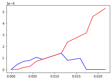
However, the chromatic aberration correction parameters have me stumped. According to exiftool there are 32 such coefficients each of which is a 16-bit integer. Examples of these coefficients, all extracted from photos taken with a Sony FE 50mm F1.8 lens are:

• F22, 30m focus: 0 128 256 384 384 384 256 256 256 256 128 128 0 0 -128 -384 0 -256 -384 -512 -512 -512 -512 -384 -384 -256 -256 -128 -128 0 128 256
• F7.1, 35m focus: 0 128 256 256 384 384 384 256 256 256 128 128 0 -128 -256 -384 0 -128 -256 -384 -384 -384 -384 -384 -384 -256 -256 -128 0 128 256 384
• F1.8, 1m focus: -384 -128 0 128 128 0 -128 0 0 0 0 0 0 0 0 0 128 -128 -256 -384 -384 -256 -256 -256 -256 -256 -256 -128 -128 0 0 0
• F2, 0.6m focus: 128 0 0 0 0 0 0 0 0 0 0 0 128 128 128 0 0 -128 -256 -384 -512 -384 -384 -384 -384 -256 -256 -256 -256 -128 -128 0

Initially, I thought that these coefficients may define a pair of splines (either concatenated together, one after the other, or with their coefficients interlaced), one describing the shift in the red channel and the other describing the shift in the blue channel. However, inspecting the coefficients quickly throws water on thus, and the resulting curves are not look sensible. This idea is also killed off by the large run of zeros which likely rules out a PCM type of interpretation. I’ve also toyed with the idea of cumulative sums, although the resulting curves did not appear to be physical.

I’ve also considered the possibility that they might be monomial coefficients for a polynomial, however, these polynomials would be exceptionally high order. Even the Adobe CA model as described in http://download.macromedia.com/pub/labs/lensprofile_creator/lensprofile_creator_cameramodel.pdf only uses 12 coefficients whereas we have 32.

As such I was wondering if anyone is aware of any other CA correction models (beyond those used by Adobe and Hugin) which might be being used here?

[Entropy512 (Andy Dodd)]

A lot of good questions… Unfortunately I’m not able to answer them, but I’m really curious to see the progress you make.

I’ve wanted to have a way to convert the distortion/vignetting correction data into a model compatible with RawTherapee for a while, to handle lenses which aren’t in lensfun yet.

As a side note, a fun additional challenge: The manner in which the data is stored in EXIF does NOT match the manner in which the lens communicates with the body. I’ve got a suspicion which messages contain correction data, but if I take a shot when the lens is on a logic analyzer, I don’t see a pattern of data even remotely matching the EXIF anywhere in any of the messages.

[fdw]

So I would not be surprised if the model data used by the mount is very different to that which the camera reports in the EXIF data. Moreover, I am almost certain that the camera is performing interpolation as even the slightest change to the overall exposure yields a raw with different correction parameters.

Looking at Imaging Edge my understanding is that it does corrections on a per-channel basis. If ds contains the 16 distortion coefficients, cr contains the first 16 CA coefficients and cb contains the final 16 CA coefficients then we have:

fpg, fpb, fpr = [], [], []
for g, b, r in zip(ds, cb, cr):
    ffpg = g*0.00006104 + 1.0
    ffpb = (b*0.00781250*0.00006104 + 1.0)*ffpg
    ffpr = (r*0.00781250*0.00006104 + 1.0)*ffpg
    
    fpg.append(ffpg)
    fpb.append(ffpb)
    fpr.append(ffpr)

In terms of the ‘magic’ numbers 0.00006104 is 2**-14 which is in agreement with the analysis in Sony ARW distortion correction, Stannum and 0.00781250 is 2**-7 for an overall scaling on the CA parameters of 2**-21. However, I am still not entirely sure how to interpret the CA coefficient arrays as plotting them does not reveal anything intuitive (or which readily matches known CA measurements for lenses).

[Entropy512 (Andy Dodd)]

Interesting - imaging edge desktop, or mobile? Looks like you used a decompiler (I’m surprised for IEM that particular code is still Java and not native, unless you have a decompiler/disassembler that does arm64/elf)

[fdw]

Desktop so 64-bit x86 which is relatively easy to debug on Windows. Pause immediately after a file has been read in, and search for the 16-bit coefficients listed by exiftool. Then set up hardware breakpoints on read and resume execution. Immediately break at the function which does the preprocessing to get them into arrays of double precision numbers.

The same function then appears to start doing a reduction over the entries in these arrays, computing the max of an expression I am still trying to unpick. However, I believe its purpose is to perform the offsetting as described in Sony ARW distortion correction, Stannum. It does not seem like this offsetting changes the arrays, however, so it might not be part of the model but rather just how Sony goes about applying the correction (a bit like the d argument in lensfun).

[Entropy512 (Andy Dodd)]

Based on the pseudocode you provided, it looks like the CA parameters “finetune” the base “green” distortion spline with an additional color-specific offset, to create three separate color-specific distortion splines, one each for b, g, and r

[JackH]

Hi fdw,

The new semi-open source Raspberry HQ Cam sports a Sony sensor (IMX477). The Foundation is pushing an open source driver called libcamera. Looking at its documentation provides hints as to what happens in Sony sensors in consumer cameras. See for instance section 5.9 here.

HIH
Jack

[fdw]

That has been my working assumption, and would make intuitive sense. However, the resulting corrections do not seem to match particularly well with external references or fit with my understanding of CA.

For example, a shot taken with a 70-200 GM at 200mm f2.8 with 240m focus distance has CA parameters: 128 0 -128 -128 -256 -256 -256 -256 -256 -384 -384 -384 -384 -512 -512 -512 -768 -640 -512 -384 -384 -256 -256 -256 -256 -128 -128 -128 0 0 0 0. Now, let us take the distortion to be 0 such that we can just correct the CA (and this appears to be what Imaging Edge does if distortion correction is disabled).

Our arrays are thus:

   fpg = [1, 1, 1, 1, 1, 1, 1, 1, 1, 1, 1, 1, 1, 1, 1, 1]
   fpr = [1.00006104, 1.0, 0.99993896, 0.99993896, 0.99987792, 0.99987792, 0.99987792, 0.99987792, 0.99987792, 0.99981688, 0.99981688, 0.99981688, 0.99981688, 0.99975584, 0.99975584, 0.9997558]
   fpb = [0.99963376, 0.9996948, 0.99975584, 0.99981688, 0.99981688, 0.99987792, 0.99987792, 0.99987792, 0.99987792, 0.99993896, 0.99993896, 0.99993896, 1.0, 1.0, 1.0, 1.0]

Taking x = np.linspace(0, np.hypot(36.0, 24.0) / 2 / 1e3, 16) and plotting as plt.plot(x, x-x*np.array(fpb), 'b-', x, x-x*np.array(fpr), 'r-') I obtain:

Ignoring the scale for the moment, we can consider comparing this to what DxOMark measured for this lens:

Here we see that past about 70% of the frame they observe a sign flip in the blue channel. However, this is not supported by the CA arrays where no sign flips occur in this region. Now, I am not going to claim DxOMark is gospel, however, it does pose some questions.

[Yakov (Yakov Galka)]

Hi, I’m the author of the linked article, and I want to confirm that to my best understand the CA coefficients are indeed corrections to the lens distortion that are to be applied as in the code you posted. Then each of the RGB planes would be warped using each of those splines (fpr, fpg, fpb).

@fdw

The same function then appears to start doing a reduction over the entries in these arrays, computing the max of an expression I am still trying to unpick

My hypothesis is that they prefer to ‘stretch’ pixels rather than ‘compress’ them. For that purpose they want fpr, fpg, fpb <= 0, which is achieved by subtracting the maximum of them all.

@fdw

the resulting corrections do not seem to match particularly well with external references or fit with my understanding of CA.

I tried to recover the CA coefficients from the camera JPEGs using the same method I described in the article. For example:

The general shape seems to more or less match, which confirms that those could be the curves that Sony’s cameras use for corrections internally.

Hope this helps!

[fdw]

@Yakov

My hypothesis is that they prefer to ‘stretch’ pixels rather than ‘compress’ them. For that purpose they want fpr, fpg, fpb <= 0 , which is achieved by subtracting the maximum of them all.

It is an interesting idea. However, what I am having trouble understanding is how this makes it possible to correct all types of distortion. Given an undistorted location (x,y) we want a function that tells us where to sample our distorted image at (xd, yd). Now, clearly we will get into trouble if for any (x,y) there is an (xd, xd) that is outside the bounds of our distorted image.

Subtracting off the max value such that (xd^2 + yd^2) < (x^2 + y^2) will clearly avoid this issue. But does it not also make it impossible to correct certain types of distortion? If we take the center of our frame to be at (0, 0) and consider a pixel (x, 0) with x > 0 it follows that we will always sample the distorted image at a point xd < x. But what if the distortion in the lens pushes things in the other direction?

Further, would this operation not be overkill in the sense that the only place where we can get into trouble with positive entries is near the edge of the frame? Hence, positive entries in the middle of the array would appear to be fine to me.

[Entropy512 (Andy Dodd)]

@fdw

But what if the distortion in the lens pushes things in the other direction?

Further, would this operation not be overkill in the sense that the only place where we can get into trouble with positive entries is near the edge of the frame? Hence, positive entries in the middle of the array would appear to be fine to me.

If the distortion is in the other direction, all of the numbers get renormalized.

As to being overkill - I’d need to think more, but yeah, this is probably nonoptimal in some scenarios (shrinking an image where it doesn’t need to be shrunk)

One thing I will say is - the rough shape of the CA curves in your plot looks similar to the DxO graph. As to the exact sign flip - there might be some residual math error somewhere.

In the DxO graph, you can see that the second derivative of the red graph is consistently increasing. The second derivative of the blue graph is consistently decreasing, except maybe near the very end. Same for your plot, same for the scaling factors themselves. (For the most part, obviously it’s a bit noiser in your data)

The one oddity is that both red and blue seem to be offset in your data (compared to DxO’s) by a positive slope of some sort. e.g. the second derivative is mostly consistent between all graphs but the first derivative has a constant positive offset, especially for red.

Do you have the original distortion correction coefficients for that shot? Perhaps there’s just a false assumption about how CA coefficients are applied when distortion correction is not?

[Entropy512 (Andy Dodd)]

Jack - that document says nothing about distortion correction .

Most of the what it does cover isn’t of significant surprise to anyone who has worked in the bowels of image processing software. For example, “lens shading correction” = “flat field correction” in RawTherapee. Similarly, “color correction matrices” is How to create DCP color profiles - RawPedia

In general the entire document is specific to fixed-lens cameras, and doesn’t really have anything for an interchangeable lens camera.

[fdw]

The associated distortion coefficients were 0 2 7 18 32 52 75 102 135 173 214 261 313 370 431 500.

In order to confirm my analysis I decompiled the relevant portion of the function. The code is a bit clunky but here goes:

dVar20 = 0.00006104; dVar21 = 1.00000000; dVar23 = 0.00781250;
do {
  cVar3 = FUN_140228d50();  // If dist correction enabled
  dVar14 = dVar21;
  if (cVar3 != '\0') {
    dVar14 = (double)(int)*(short *)(*(longlong *)(param_2 + 0x12c0) + lVar9) * dVar20 + dVar21;
  }
  cVar3 = FUN_140228d70();  // If CA correction enabled
  dVar17 = dVar21;
  dVar18 = dVar21;
  if (cVar3 != '\0') {
    dVar17 = (double)(int)*(short *)(*(longlong *)(param_2 + 0x12d0) + lVar9) * dVar23 * dVar20
             + dVar21;
    dVar18 = (double)(int)*(short *)(*(longlong *)(param_2 + 0x12d8) + lVar9) * dVar23 * dVar20
             + dVar21;
  }
  *(double *)(lVar11 + *(longlong *)(param_1 + 4)) = dVar14;            // fpg
  *(double *)(lVar11 + *(longlong *)(param_1 + 2)) = dVar17 * dVar14;   // fpr
  *(double *)(lVar11 + *(longlong *)(param_1 + 6)) = dVar18 * dVar14;   // fpb
  iVar12 = iVar12 + 1; lVar9 = lVar9 + 2; lVar11 = lVar11 + 8;
} while (iVar12 < *param_1);

Notice how dVar14 which contains the distortion correction entry starts off at 1.0. Another thing I am reasonably confident in is that these arrays which are being assigned here do not change and are subsequently accessed by a hot loop. (And what is being computed by the remainder of this function is a scalar which goes into param_1 + 8.)

[JackH]

Gotcha Andy, not my area of expertise, I was hoping there would be something interesting in there for you.

[Entropy512 (Andy Dodd)]

As far as your plot of the R/B corrections - I get this (albeit with a different scaling factor, and I attempted to do a spline interpolation):

I do see the sign change for blue that is seen in the DxO numbers, and the blue flattening/reversing its slope near the end (obviously, here, it’s a more aggressive reversal)

What I see inconsistent is that instead of being consistently positive, red starts negative and shifts positive later.

Edit: Note that I started with your fpr/fpb arrays, instead of calculating them from scratch. But this looks a little weird to me:

Your first red entry is 128 (not 0), but your first entry in fpr is 1.0?

[fdw]

Sorry! That was a copy and paste typo on my end which I have now corrected. The floating point values should now be correct.

[Entropy512 (Andy Dodd)]

Yup. I’m now getting similar plots to you.

Still, it generally does appear that the shapes of the curves are reasonably similar. Red consistently increases (and the slope increases with radius), while blue starts out sloping upwards with radius, but then slopes downwards before leveling off.

[fdw]

So as a cross check I’ve also looked at the Sony 24-70 GM lens at 24mm F2.8. Here I find the coefficients to be: 384 384 384 512 512 512 512 512 512 512 640 640 640 768 768 1024 -128 0 128 256 384 384 512 512 384 384 384 256 256 128 0 0 and the distortion coefficients to be: 13 0 -23 -52 -92 -137 -192 -248 -307 -363 -419 -464 -501 -519 -521 -489. Neglecting the distortion and just considering the CA I obtain the following plot:

By comparison this is what DxOMark reports:

This is also a lens which has been profiled and is in the lensfun database with the entry:
<tca model="poly3" focal="24" vr="1.0001797" vb="1.0001569"/>
with the corresponding model being described here:
https://lensfun.github.io/manual/latest/group__Lens.html#ga0b8deda1887fb5543a2038669ed344b4

These values work reasonably well for me and do a reasonable job at reducing CA (although they are not as clean as the camera JPEG’s when corrections are enabled). Note, however, that vr and vb are not too dissimilar; at least certainly not to the extent of the measurements by DxOMark .

[fdw]

So I’ve been thinking about this problem some more, and debugging a bunch more code. As such, I am now quite confident in my interpretation of the various arrays - even if the results are in contradiction with the data in other sources.

To this end for the 24-70mm GM lens at 24mm f2.8 I’ve done a curve fit of the coefficients for the third order TCA model employed by lensfun against the spline extracted from the RAW file. Here I find:
<tca model="poly3" focal="24" vr="1.00031063" vb="1.00004585" cr="-2.03134916e-04" cb="3.60076934e-04" br="1.33663750e-04" bb="-2.00643975e-04" />

In terms of results the below image shows a tight 400% crop from the top left of a snapshot with no CA correction:

Here, we can see some clear CA. With the existing profile in lensfun (shown in my previous post) we obtain:

The result is a clear improvement, albeit with some slight halos. With my extracted coefficients we obtain:

To my eyes this is a slight improvement with the slight green-purple fringe replaced by a yellow-blue fringe which seems a bit softer.

I still need to do some more validation with other lenses, but these results are quite encouraging.

I also believe I have a reasonable handle on vignetting correction, although it might be a few more days before I am in a position to convert these splines into lenfun models.

[Entropy512 (Andy Dodd)]

Figuring out the curve fitting is the main reason I haven’t tried implementing this in RT.

Your results provide significant additional motivation to do this - it’s clear that for this lens (and probably most Sony first-party lenses), the built-in profile data is better than what most people can measure and provide to lensfun.