Sony RAW Chromatic Aberration Correction Model

Yup. I’m now getting similar plots to you.

Still, it generally does appear that the shapes of the curves are reasonably similar. Red consistently increases (and the slope increases with radius), while blue starts out sloping upwards with radius, but then slopes downwards before leveling off.

So as a cross check I’ve also looked at the Sony 24-70 GM lens at 24mm F2.8. Here I find the coefficients to be: 384 384 384 512 512 512 512 512 512 512 640 640 640 768 768 1024 -128 0 128 256 384 384 512 512 384 384 384 256 256 128 0 0 and the distortion coefficients to be: 13 0 -23 -52 -92 -137 -192 -248 -307 -363 -419 -464 -501 -519 -521 -489. Neglecting the distortion and just considering the CA I obtain the following plot:
index

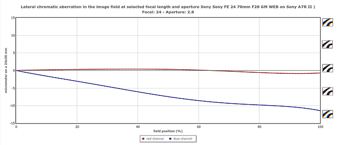
By comparison this is what DxOMark reports:

This is also a lens which has been profiled and is in the lensfun database with the entry:
<tca model="poly3" focal="24" vr="1.0001797" vb="1.0001569"/>
with the corresponding model being described here:
https://lensfun.github.io/manual/latest/group__Lens.html#ga0b8deda1887fb5543a2038669ed344b4

These values work reasonably well for me and do a reasonable job at reducing CA (although they are not as clean as the camera JPEG’s when corrections are enabled). Note, however, that vr and vb are not too dissimilar; at least certainly not to the extent of the measurements by DxOMark .

1 Like

So I’ve been thinking about this problem some more, and debugging a bunch more code. As such, I am now quite confident in my interpretation of the various arrays - even if the results are in contradiction with the data in other sources.

To this end for the 24-70mm GM lens at 24mm f2.8 I’ve done a curve fit of the coefficients for the third order TCA model employed by lensfun against the spline extracted from the RAW file. Here I find:
<tca model="poly3" focal="24" vr="1.00031063" vb="1.00004585" cr="-2.03134916e-04" cb="3.60076934e-04" br="1.33663750e-04" bb="-2.00643975e-04" />

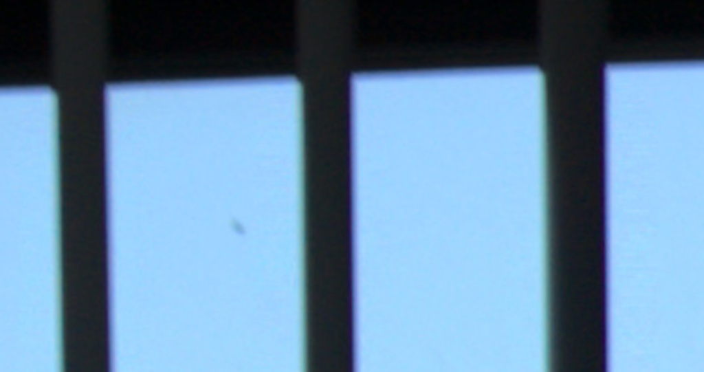
In terms of results the below image shows a tight 400% crop from the top left of a snapshot with no CA correction:


Here, we can see some clear CA. With the existing profile in lensfun (shown in my previous post) we obtain:

The result is a clear improvement, albeit with some slight halos. With my extracted coefficients we obtain:

To my eyes this is a slight improvement with the slight green-purple fringe replaced by a yellow-blue fringe which seems a bit softer.

I still need to do some more validation with other lenses, but these results are quite encouraging.

I also believe I have a reasonable handle on vignetting correction, although it might be a few more days before I am in a position to convert these splines into lenfun models.

3 Likes

Figuring out the curve fitting is the main reason I haven’t tried implementing this in RT.

Your results provide significant additional motivation to do this - it’s clear that for this lens (and probably most Sony first-party lenses), the built-in profile data is better than what most people can measure and provide to lensfun.

So I’ve started putting some code together. For all of the base polynomials used by lensfun the coefficients can be determined exactly through the solution of a suitably framed linear least squares problem (this is important, as non-linear least squares is a real pain and seldom suitable for real-time applications).

I’ve done a first pass of almost everything except for the distortion molestation routine. This is responsible from converting the coefficients from their natural form to that used by the lensfun database (the irony being that not too long after reading these coefficients in lensfun undoes these transforms to return the polynomial back to its natural form). Finishing this routine will require me to write a full multi-variate implementation of Newton’s method. That and a huge amount of testing and debugging.

#include <stdio.h>
#include <tgmath.h>

static inline
void givens(double f, double g, double *c, double *s)
{
    if (g == 0.0)
    {
        *c = 1.0;
        *s = 0.0;
    }
    else if (f == 0.0)
    {
        *c = 0.0;
        *s = copysign(1.0, g);
    }
    else
    {
        double l = sqrt(f*f + g*g);
        *c = fabs(f) / l;
        *s = copysign(1.0, f)*g / l;
    }
}

static inline
void givens_qr(double *A, double *b, int m, int n)
{
    for (int j = 0; j < n; j++)
    {
        for (int i = m - 1; i > j; i--)
        {
            int k = i - 1;
            
            double c, s;
            givens(A[k*n + j], A[i*n + j], &c, &s);
            
            // Apply to A
            for (int l = j; l < n; l++)
            {
                double p = A[k*n + l], q = A[i*n + l];
                A[k*n + l] =  c*p + s*q;
                A[i*n + l] = -s*p + c*q;
            }
            
            // Apply to b
            double p = b[k], q = b[i];
            b[k] =  c*p + s*q;
            b[i] = -s*p + c*q;
        }
    }
}

static inline
void solve_bwd(double *R, double *b, double *x, int n)
{
    for (int i = n - 1; i >= 0; i--)
    {
        double t = b[i];
        
        for (int j = i + 1; j < n; j++)
            t -= R[i*n + j]*x[j];
        
        x[i] = t / R[i*n + i];
    }
}

static inline
void interpolate(double *spcoeffs, int nc, double *xv, double *yv, int m)
{
    for (int i = 0; i < m; i++)
    {
        xv[i] = (double) i / (m - 1);
        
        for (int j = 1; j < nc; j++)
        {
            double l = (j - 1.0) / (nc - 1), r = (double) j / (nc - 1);
            
            if (xv[i] >= l && xv[i] <= r)
            {
                double dydx = (nc - 1)*(spcoeffs[j] - spcoeffs[j - 1]);
                
                yv[i] = spcoeffs[j - 1] + (xv[i] - l)*dydx;
                break;
            }
        }
    }
}

int
train_sony_dist(const short *coeffs, int nc, double tcoeffs[3])
{
    enum { M = 128, N = 3 };
    
    // Check the coefficient count
    if (nc != 16)
       return -1;
    
    // Pre-process the coefficients
    double spcoeffs[16];
    for (int i = 0; i < nc; i++)
        spcoeffs[i] = coeffs[i]*pow(2.0, -14.0) + 1.0;
    
    // Interpolate the resulting spline onto a fine grid
    double xv[M], yv[M];
    interpolate(spcoeffs, 16, xv, yv, M);
    
    // Form the A matrix and b vector
    double A[M*N], b[M];
    for (int i = 0; i < M; i++)
    {
        A[i*N + 0] = pow(xv[i], 1);
        A[i*N + 1] = pow(xv[i], 2);
        A[i*N + 2] = pow(xv[i], 3);
        
        b[i] = yv[i] - 1.0;
    }
    
    // Solve the linear least squares problem
    givens_qr(A, b, M, N);
    solve_bwd(A, b, tcoeffs, N);
    
    return 0;
}

void
molest_sony_dist(double fl, const double tcoeffs[3], double mcoeffs[3])
{
    //double hugin_scale = fl / (hypot(36.0, 24.0) / hypot(1.5, 1.0) / 2.0);
    
    // TODO: This needs Newton's method
}

int
train_sony_tca(const short *coeffs, int nc, double tcoeffs[3])
{
    enum { M = 64, N = 3 };
    
    // Check the coefficient count
    if (nc != 16)
       return -1;
    
    // Pre-process the coefficients
    double spcoeffs[16];
    for (int i = 0; i < nc; i++)
        spcoeffs[i] = coeffs[i]*pow(2.0, -21.0) + 1.0;
    
    // Interpolate the resulting spline onto a fine grid
    double xv[M], yv[M];
    interpolate(spcoeffs, 16, xv, yv, M);
    
    // Form the A matrix and b vector
    double A[M*N], b[M];
    for (int i = 0; i < M; i++)
    {
        A[i*N + 0] = 1.0;
        A[i*N + 1] = pow(xv[i], 1);
        A[i*N + 2] = pow(xv[i], 2);
        
        b[i] = yv[i];
    }
    
    // Solve the linear least squares problem
    givens_qr(A, b, M, N);
    solve_bwd(A, b, tcoeffs, N);
    
    return 0;
}

void
molest_sony_tca(double fl, const double tcoeffs[3], double mcoeffs[3])
{
    double hugin_scale = fl / (hypot(36.0, 24.0) / hypot(1.5, 1.0) / 2.0);
    mcoeffs[0] = tcoeffs[0];
    mcoeffs[1] = tcoeffs[1] / hugin_scale;
    mcoeffs[2] = tcoeffs[2] / (hugin_scale*hugin_scale);
}

int
train_sony_vig(const short *coeffs, int nc, double tcoeffs[3])
{
    enum { M = 128, N = 3 };
    
    // Check the coefficient count
    if (nc != 16)
       return -1;
    
    // Pre-process the coefficients
    double spcoeffs[16];
    for (int i = 0; i < nc; i++)
        spcoeffs[i] = pow(2.0, pow(2.0, pow(2.0, -13.0)*coeffs[i]) - 1.0);
    
    // Interpolate the resulting spline onto a fine grid
    double xv[M], yv[M];
    interpolate(spcoeffs, 16, xv, yv, M);
    
    // Form the A matrix and b vector
    double A[M*N], b[M];
    for (int i = 0; i < M; i++)
    {
        /*
         * Place a strong emphasis on getting the final point correct.
         */
        double wgt = (i == M - 1) ? 25.0 : 1.0;
        
        A[i*N + 0] = wgt*pow(xv[i], 2.0);
        A[i*N + 1] = wgt*pow(xv[i], 4.0);
        A[i*N + 2] = wgt*pow(xv[i], 6.0);
        
        b[i] = wgt*(1.0 / yv[i] - 1.0);
    }
    
    // Solve the linear least squares problem
    givens_qr(A, b, M, N);
    solve_bwd(A, b, tcoeffs, N);
    
    return 0;
}

int
main()
{
    // Test TCA
    double vcb[3], mvcb[3];
    short coeffs[] = { 384, 384, 384, 512, 512, 512, 512, 512, 512, 512, 640, 640, 640, 768, 768, 1024 };
    
    train_sony_tca(coeffs, 16, vcb);
    molest_sony_tca(24.0, vcb, mvcb);
    
    printf("TCA: v = %f\tc = %e\tb = %e\n", mvcb[0], mvcb[1], mvcb[2]);
    
    // Test vignetting
    double k123[3];
    short vcoeffs[] = { 0, 32, 128, 288, 480, 736, 1056, 1376, 1984, 3360, 5024, 6560, 8128, 9728, 11360, 13184 };
    
    train_sony_vig(vcoeffs, 16, k123);
    
    printf("Vig: k1 = %f\tk2 = %f\tk3 = %f\n", k123[0], k123[1], k123[2]);
    
    return 0;
}
1 Like

Hi, this is very cool! How do you plan to license the code?

Thanks!

I’ve updated the code to include the distortion coefficient molestation routine. In my testing this appears to converge reasonably reliably, although a huge amount more testing is needed. I also removed support for interpolation as, on reflection, it did not appear to be helping.

#include <stdio.h>
#include <tgmath.h>

static inline
void givens(double f, double g, double *c, double *s)
{
    if (g == 0.0)
    {
        *c = 1.0;
        *s = 0.0;
    }
    else if (f == 0.0)
    {
        *c = 0.0;
        *s = copysign(1.0, g);
    }
    else
    {
        double l = sqrt(f*f + g*g);
        *c = fabs(f) / l;
        *s = copysign(1.0, f)*g / l;
    }
}

static inline
void givens_qr(double *A, double *b, int m, int n)
{
    for (int j = 0; j < n; j++)
    {
        for (int i = m - 1; i > j; i--)
        {
            int k = i - 1;
            
            double c, s;
            givens(A[k*n + j], A[i*n + j], &c, &s);
            
            // Apply to A
            for (int l = j; l < n; l++)
            {
                double p = A[k*n + l], q = A[i*n + l];
                A[k*n + l] =  c*p + s*q;
                A[i*n + l] = -s*p + c*q;
            }
            
            // Apply to b
            double p = b[k], q = b[i];
            b[k] =  c*p + s*q;
            b[i] = -s*p + c*q;
        }
    }
}

static inline
void solve_bwd(const double *R, const double *b, double *x, int n)
{
    for (int i = n - 1; i >= 0; i--)
    {
        double t = b[i];
        
        for (int j = i + 1; j < n; j++)
            t -= R[i*n + j]*x[j];
        
        x[i] = t / R[i*n + i];
    }
}

int
train_sony_dist(const short *coeffs, int nc, double tcoeffs[3])
{
    // Check the coefficient count
    if (nc != 16)
       return -1;
    
    // Pre-process the coefficients
    double xv[16], yv[16];
    for (int i = 0; i < nc; i++)
    {
        xv[i] = (double) i / (nc - 1);
        yv[i] = coeffs[i]*pow(2.0, -14.0) + 1.0;
    }
        
    // Form the A matrix and b vector
    double A[16*3], b[16];
    for (int i = 0; i < nc; i++)
    {
        A[i*3 + 0] = xv[i];
        A[i*3 + 1] = xv[i]*xv[i];
        A[i*3 + 2] = xv[i]*xv[i]*xv[i];
        
        b[i] = yv[i] - 1.0;
    }
    
    // Solve the linear least squares problem
    givens_qr(A, b, nc, 3);
    solve_bwd(A, b, tcoeffs, 3);
    
    return 0;
}

void
molest_sony_dist(double fl, const double tcoeffs[3], double mcoeffs[3])
{
    const double hs = fl / (hypot(36.0, 24.0) / hypot(1.5, 1.0) / 2.0);
    const double at = tcoeffs[2], bt = tcoeffs[1], ct = tcoeffs[0];
    
    // Scratch space
    double r[3], s[3], J[9];
    
    // Initial guess of the molested coefficients
    double am = at / (hs*hs*hs);
    double bm = bt / (hs*hs);
    double cm = ct / hs;
    
    for (int i = 0; i < 5; i++)
    {
        double d = 1 - am - bm - cm;
        
        // Evaluate the residual
        r[0] = am*hs*hs*hs / (d*d*d*d) - at;
        r[1] = bm*hs*hs / (d*d*d) - bt;
        r[2] = cm*hs / (d*d) - ct;
        
        // Form the Jacobian matrix
        J[0] = J[1] = J[2] = 4.0*am*hs*hs*hs / (d*d*d*d*d);
        J[3] = J[4] = J[5] = 3.0*bm*hs*hs / (d*d*d*d);
        J[6] = J[7] = J[8] = 2.0*cm*hs / (d*d*d);
        
        J[0] += pow(hs, 3.0) / (d*d*d*d);
        J[4] += pow(hs, 2.0) / (d*d*d);
        J[8] += hs / (d*d);
        
        // Solve the resulting linear system
        givens_qr(J, r, 3, 3);
        solve_bwd(J, r, s, 3);
        
        // Update our guesses for the molested coefficients
        am -= s[0];
        bm -= s[1];
        cm -= s[2];
    }
    
    mcoeffs[0] = cm;
    mcoeffs[1] = bm;
    mcoeffs[2] = am;
}

int
train_sony_tca(const short *coeffs, int nc, double tcoeffs[3])
{
    // Check the coefficient count
    if (nc != 16)
       return -1;
    
    // Pre-process the coefficients
    double xv[16], yv[16];
    for (int i = 0; i < nc; i++)
    {
        xv[i] = (double) i / (nc - 1);
        yv[i] = coeffs[i]*pow(2.0, -21.0) + 1.0;
    }
    
    // Form the A matrix and b vector
    double A[16*3], b[16];
    for (int i = 0; i < nc; i++)
    {
        A[i*3 + 0] = 1.0;
        A[i*3 + 1] = xv[i];
        A[i*3 + 2] = xv[i]*xv[i];
        
        b[i] = yv[i];
    }
    
    // Solve the linear least squares problem
    givens_qr(A, b, nc, 3);
    solve_bwd(A, b, tcoeffs, 3);
    
    return 0;
}

void
molest_sony_tca(double fl, const double tcoeffs[3], double mcoeffs[3])
{
    const double hs = fl / (hypot(36.0, 24.0) / hypot(1.5, 1.0) / 2.0);
    mcoeffs[0] = tcoeffs[0];
    mcoeffs[1] = tcoeffs[1] / hs;
    mcoeffs[2] = tcoeffs[2] / (hs*hs);
}

int
train_sony_vig(const short *coeffs, int nc, double tcoeffs[3])
{
    // Check the coefficient count
    if (nc != 16)
       return -1;
    
    // Pre-process the coefficients
    double xv[16], yv[16];
    for (int i = 0; i < nc; i++)
    {
        xv[i] = (double) i / (nc - 1);
        yv[i] = pow(2.0, pow(2.0, pow(2.0, -13.0)*coeffs[i]) - 1.0);
    }
    
    // Form the A matrix and b vector
    double A[16*3], b[16];
    for (int i = 0; i < nc; i++)
    {
        A[i*3 + 0] = xv[i]*xv[i];
        A[i*3 + 1] = xv[i]*xv[i]*xv[i]*xv[i];
        A[i*3 + 2] = xv[i]*xv[i]*xv[i]*xv[i]*xv[i]*xv[i];
        
        b[i] = 1.0 / yv[i] - 1.0;
    }
    
    // Solve the linear least squares problem
    givens_qr(A, b, nc, 3);
    solve_bwd(A, b, tcoeffs, 3);
    
    return 0;
}

int
main()
{
    /*// Test TCA
    double vcb[3], mvcb[3];
    short coeffs[] = { 384, 384, 384, 512, 512, 512, 512, 512, 512, 512, 640, 640, 640, 768, 768, 1024 };
    
    train_sony_tca(coeffs, 16, vcb);
    molest_sony_tca(24.0, vcb, mvcb);
    
    printf("TCA: v = %f\tc = %e\tb = %e\n", mvcb[0], mvcb[1], mvcb[2]);*/
    
    // Test vignetting
    /*double k123[3];
    short vcoeffs[] = { 0, 32, 128, 288, 480, 736, 1056, 1376, 1984, 3360, 5024, 6560, 8128, 9728, 11360, 13184 };
    
    train_sony_vig(vcoeffs, 16, k123);
    
    printf("Vig: k1 = %f\tk2 = %f\tk3 = %f\n", k123[0], k123[1], k123[2]);*/
    
    double cab[] = { 0.012336653221805166, -0.14320916760453498, 0.10035892348474476 };
    double mcab[3];
    molest_sony_dist(24.0, cab, mcab);
    
    printf("%f\t%f\t%f\n", mcab[2], mcab[1], mcab[0]);
    
    return 0;
}

I am happy for the code to be BSD licensed.

This makes me wonder if attempting to do a curve fit is the right approach, vs. trying to integrate a new model into lensfun?

@heckflosse and @Morgan_Hardwood - who is most familiar with the lensfun integration in RT? Any thoughts on the best architecture for this?

@agriggio implemented lensfun integration in RT

I would like to see a comparison between this method and the raw auto-ca-correction in RT.

For the test shots I have to hand I find them to be about the same; which is not entirely surprising. Of the three major types of distortion TCA is usually the easiest to correct. However, the advantage of this approach is that it can also pull out the distortion and vignetting coefficients. These can both be very difficult to determine on the fly for a general picture. Moreover, for TCA this gets the coefficients in one shot with very little computational effort.

Could you provide a raw file for comparison please?

Here is a shot taken with a 24-105mm lens at F4 at 24mm. It shows a lot of distortion and vignetting, along with a small amount of TCA:

_DSC1633.ARW (42.0 MB)

Running this through my code I obtain the following lensfun profile:

    <distortion model="ptlens" focal="24" a="0.010061" b="-0.035326" c="0.002272"/>
    <tca model="poly3" focal="24" vr="1.000425" vb="1.000260" />
    <vignetting model="pa" focal="24.0" aperture="4.0" distance="10" k1="-0.105723" k2="-1.112484" k3="0.461957" />
    <vignetting model="pa" focal="24.0" aperture="4.0" distance="1000" k1="-0.105723" k2="-1.112484" k3="0.461957" />

which when brought into DT (my version of RT has trouble identifying the lens) corrects up reasonably nicely. I note that these coefficients are different to those which already exist in the current release of lensfun for this lens lensfun/mil-sony.xml at master · lensfun/lensfun · GitHub although would not necessarily read too much into this.

This alone likely is a significant benefit - merely not having to auto-characterize the CA because the actual properties of the lens are stored in the image metadata itself.

Can these be fed into pre-demosaic CA correction somehow?

pre-demosaic CA correction changes only red and blue raw channels. Does the new method also changes green?

Yes, this method can give you the CA correction curves for the red and blue channels.

If you also have distortion correction enabled - yes, it effectively implements CA correction by implementing different DC curves for each channel.

However, to facilitate operating without DC, the CA curves are encoded as deltas from the green DC curve, so you can apply just those deltas to do CA correction without distortion correction.

To throw something of a spanner in the works whilst working on adding support for coefficient extraction in Exiv2 I found that the coefficients my code was extracting did not agree precisely with those of Exiftool. After a bit more poking around it appears as if Sony cameras store two sets of coefficients. For the ARW file I uploaded in a previous post we find

[SubIFD]        DistortionCorrParams            : 16 13 -2 -29 -65 -113 -171 -241 -313 -394 -473 -557 -636 -713 -780 -841 -884
[Sony]          DistortionCorrParams            :    14 -2 -32 -72 -126 -190 -268 -348 -438 -526 -620 -708 -794 -868 -936 -984
[Sony]          DistortionCorrParams            :    14 -2 -32 -72 -126 -190 -268 -348 -438 -526 -620 -708 -794 -868 -936 -984
[SR2SubIFD]     DistortionCorrParams            : 16 13 -2 -29 -65 -113 -171 -241 -313 -394 -473 -557 -636 -713 -780 -841 -884

By default we’ve been seeing those in SubIFD/SR2SubIFD and it appears to be those which ImagingEdge (at least the version I inspected) uses. However, it would be good to know if anyone has any insight around the second set of coefficients and if they are subject to the same interpretation as the first set or not.