right, these come straight out of the neutral fitter. i was hoping to hide them from the ui/show only in some advanced setting and only display the tune counterparts. the final filter weight is then just filter m + tune m * 0.1 and clamped to [0,1].
The 2383 definitely has a look, which is why it is quite widely appreciated and used by film makers and colorists. I like the results you got with it!
Thanks @cameronrad, that’s a nice comparison.
There is already variability among those three sources.
I wonder how are this LUTs made? Do you have any insight about that?
Since the look of print paper (or print film) is really achieved only after projecting a negative, I wonder how they can isolate the LUT for only the final printing medium. I guess severe assumptions on the input need to be made. Or maybe “Vision3 input” is somehow assumed.
2383 looks somewhat warmer and more stylized also in your comparisons, from Koji and Adobe. That is a good sign, and it aligns with the results we get from agx-emulsion and the data from the technical documents.
When you say that the LUT is optimized for a white point, do you mean that neutral gray input is giving a different tint at the output according to the white point?
now that most of the agx-emulsion pipeline is implemented in vkdt, i’m going over it once more in more detail to find differences and find out which of these are problems or just different…
i’m still unsure whether my noise model is comparable to yours, doing some more tests on a synthetic ramp (worth pointing out that this runs through a virtual ND filter that is not a linear transmittance ramp, only for the left half or so it’s close).
i use a procedural noise pattern to compute the variation of grain numbers in each pixel. this is kinda the poisson part. then i use a binomial to sample whether or not these grains turn. the binomial distribution has some built-in variance reduction at the rims, for p=0 and p=1. not sure why i can’t see this in your plots, i believe because the poission part dominates so much? or maybe because i’m using the large-N gaussian approximation for the binomial.
anyways, here are some results: the waveform histogram shows straight value, not standard deviation as your grain plots above, but you can also see how the variance compresses towards the extremes (white/black). increasing exposure of the ramp:
this is with lower uniform parameter, which means variation of the number of grains in each pixel, giving an overall more granular look. this adds another source of variance, hence the point cloud in the waveform explodes. the size of the grains makes no difference, since it’s integrated away over the height of the test strip.
this is the negative, very under exposed (-5ev) to stretch the range, shows some quantisation artifacts in the deep to-be-blacks on the right end of the test strip:
this one is with
uniform=1 but setting it to zero just increases variance overall, except for in the blacks where it stays the same as in the above image.
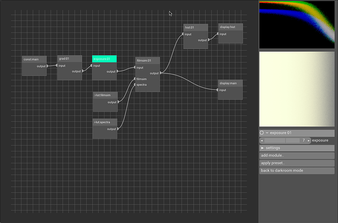
for completeness here’s the processing graph .cfg file:
test.cfg (1.6 KB)
i have to stare at these strips for a bit more, but i think the noise model might fall into the category “different but i’m happy with it”. i probably want to change the parameters around, maybe a combo box with a few ISO speed ratings.
Just a quick comment, I compiled an hour or so ago and Endura premium seems to be the only paper that looks reasonable. Now I don’t know what I’m doing with vtkd so take it with a grain of salt. The sims look kind of ok with Endura though. The other papers are very yellowish.
The grain as seen when turning on “simulate grain” looks really quite strange and nothing like the agx app. It’s very contrasty and pixly, not very analogue looking.
Also wondering if paper exposure works the same in both apps? Feels different i vktd.
I played a bit with it in vkdt, and it is quite fun to work with, but even spending lots of time, I cannot get out an image that doesn’t look “over the top”.
I’m not using the grain stuff for now and am leaving the couplers at 0 for now. Tune m and tune y seem to act as something like a white balance. So after adjusting m and y to get neutral colors, there are film and paper as well as 4 sliders remaining, of which 2 of each seem to do mostly the same thing.
Concerning film and paper, I started with Porta 400 and Porta Endura.
What does your graph in the node editor look like? I’m using this for now:
Disabling filmsim, what should the image look like? Correctly white balanced and exposed, I suppose?
I also wouldn’t mind a cfg file to compare results just to be sure there is no AMD exclusive bug involved ![]()
next up: the weird colour cast i’ve seen since the beginnig. i printed all buffers of log spectral power and density etc and compared to the corresponding agx output. of course they kinda diverge, i.e. earlier stages are more similar. the enlarger with thungsten vs 3200K and the filter transmittances make quite a bit of a difference.
turns out the initial film exposure step was calibrated to 1ev brighter on my side as it was on agx-emulsion code.
also: if density is NaN this means infinite density, not zero ![]() which was quite the change. anyways i’ll spare you with the debugging output, maybe one example, the negative of the test image:
which was quite the change. anyways i’ll spare you with the debugging output, maybe one example, the negative of the test image:
and a final render with default settings and everything fancy disabled in agx-emulsion and the corresponding vkdt render:
both use like -0.5 ev print exposure, no auto exposure. i had to tune the m and y filters in vkdt a bit, but not all that much (not aiming for best match here, just eyeballed from far away for a few seconds, you can tell by the background). now re-fitting all the neutral values, i think i can finally leave filter c at a constant and get valid values for the two others. big step towards equivalent output i think. science is only magic if it’s really completely correct…
Just judging by the waveforms the grain does seams to behave quite well, and it responds to uniformity as I would expect.
At the extremes of the density values I use density_min (i.e. the fog) to lift the variance when density (over base + fog) is close to zero, and as you mention I reduce uniformity to increase the variance close to density max. I am recalling the next plot for reference. In that simplified script I omitted density_min, but it would lift the left part of the graph.
Is this you were referring to?
As a comment, when printing on paper the effect of fog or uniformity might not be very visible. Most of the time we are printing only the “linear part” of the negative. So the behavior for p=0 or p=1, is mostly relevant for simulating underexposure or overexposure.
When comparing with real ISO speed ratings and RMS granularity I usually compute a test image with a ramp (as yours), and a pixel size equal to the area of the aperture of the densitometer used in the measurements (circular with a diameter of 48um). Standard deviation times 1000 should be tune to be close to the measured values, and for different pixel sizes we trust the particle model to scale well. The usual range of RMS granularity for color film is 5-30, depending on ISO.
This indeed can add some casts that happens with over-exposures, more strong in consumer films. Portra 400 instead is more invariant.
That is also a very good sing! According to real life, the cyan filter should also be set to zero, but I cannot really make them work in that way because I would need negative values for magenta filters.
The comparison in the portrait is also getting closer, In the example still some residual magenta tint that could be adjusted with the m-filter most likely.
I am experimenting a bit with the profile making scripts. There are a few parts that I am rethinking about the sensitivity unmixing. Especially because I want to experiment with tungsten balanced film, that I believe would not work well right now.
In the weekend I added some more film data:
- Ektar 100
- the missing ones from the Portra family: 160, 800, 800 (push 1 stop), 800 (push 2 stops)
I quite like the profile of Ektar 100 ![]()
saw that! struggling with the white balance as we speak. did you use the LED lights for 2383 and 2392 now? and how do you fit? what works best for me currently is some completely idiotic random search of the whole domain, followed by refinement with nelder mead.
Cool! I just downloaded https://github.com/andreavolpato/agx-emulsion/archive/refs/heads/main.zip but the only new film I see is kodak_vision3_50d. kodak_ektar_100 is not there as an example.
Seems it should be there according to https://github.com/andreavolpato/agx-emulsion/commit/fa5956c9aae8821a23602851452d652b7e32f0e6. Strange?
For the cine color print film I used the same 3200K (tungsten-halogen). The data looks a bit strange especially for 2393, there is some thinking to be done. It is not clear what are the experimental conditions when measuring density curves and sensitivities, and how I should take this into account to better balance the profiles and make them more compatible to the virtual enlarger.
For all the film stock I added in the enlarger a heat filter (Schott KG3), plus the transmission of a real lens, to imitate the enlarger lens. Apparently lenses with normal glass cut the UV from around 400-380 nm.
In the end the total filter looks very similar to what used in the virtual camera. So probably I will substitute it with a generic filter without relying on the actual experimental data.
I did change also the dichroic filters of the enlarger, I found a remote PDF with measurments of the real dichroics of a Durst enlarger (http://www.jollinger.com/photo/cam-coll/manuals/enlargers/durst/Durst_Enlarger_Guide.pdf). In my opinion they are better optimized for the transitions of the dyes and absorptions of the paper. Thorlabs and Edmund Optics ones are generic for a wide range of applications, and they are more “leaky”.
That is strange indeed. I see the data when downloading in the main.zip file.
I did another small commit, maybe you can try again.
I also saw @Y69 doing a very nice play raw with Ektar 100.
i don’t want to hijack arctic’s thread here, where the discussion about new film stocks and the spectral model takes place… maybe start a new thread specifically about mondane vkdt bugs? i pushed some fixes and the new films (portra family + ektar), breaking old cfg files in the process, so maybe some things are already fixed. to make the grain look really very good i think i want to look at some properties here in more detail.
hah, really nice. i think the shape of this “envelope” function looks pretty much like what i had dialed in by hand: quick slope from 380 to 400 and slower decay towards 800nm. it’s probably a difference though where the filter is applied. i have it at the very beginning of the pipeline, assuming that the wavelengths don’t exchange energy until the very end (see my comment about fluorescence), but this is incorrect. the way the density is formed totally allows for some cross talk between wavelengths, so it’s probably important to apply the filter in the print exposure stage.
…and this one is more like my smooth approximation that sums the filters to one when they transition! this way easier/more robust to fit, and i was kinda proud i could converge the thorlabs-like filters for all film/paper combinations now. i shall try the durst-like filters too.
Deleted the old agx-emulsion directory and downloaded master again. After that I ran:
uv run --python 3.11 --with-requirements requirements.txt --no-project --with-editable .
uv run --python 3.11 --with-requirements requirements.txt --no-project --with-editable . agx_emulsion/gui/main.py
Still no go. I have:
- kodak_portra_400
- kodak_ultramax_400
- kodak_gold_200
- kodak_vision3_50d
- fujifilm_pro_400h
- fujifilm_xtra_400
- fujifilm_c200
![]() I’ll wait and see if it gets solved with a later code update.
I’ll wait and see if it gets solved with a later code update.
Is anyone running this on mesa 25 and amd hardware? I use arch and I can’t get napari showing up properly. All other stuff like glxgears etc work just fine so I am really lost what I could be missing. The error is
WARNING: qglx_findConfig: Failed to finding matching FBConfig for QSurfaceFormat(version 2.0, options QFlags<QSurfaceFormat::FormatOption>(), depthBufferSize 0, redBufferSize 1, greenBufferSize 1, blueBufferSize 1, alphaBufferSize 0, stencilBufferSize 0, samples 0, swapBehavior QSurfaceFormat::SingleBuffer, swapInterval 1, colorSpace QSurfaceFormat::DefaultColorSpace, profile  QSurfaceFormat::NoProfile)
WARNING: qglx_findConfig: Failed to finding matching FBConfig for QSurfaceFormat(version 2.0, options QFlags<QSurfaceFormat::FormatOption>(), depthBufferSize 0, redBufferSize 1, greenBufferSize 1, blueBufferSize 1, alphaBufferSize 0, stencilBufferSize 0, samples 0, swapBehavior QSurfaceFormat::SingleBuffer, swapInterval 1, colorSpace QSurfaceFormat::DefaultColorSpace, profile  QSurfaceFormat::NoProfile)
WARNING: Could not initialize GLX
when using “export QT_XCB_GL_INTEGRATION=none” I get a black window which has clickable menus and stuff but I can’t see anything.
Any pointers would be highly appreciated.
Edit: Found the solution here:
https://www.reddit.com/r/NobaraProject/comments/1fb2o4v/after_updating_to_nobara40_anaconda_navigator_not/
conda install -c conda-forge libstdcxx-ng does the trick. Now on to playing ![]()
Can only speak for myself, but it doesn’t bother me that both types of conversation takes place in this thread. ![]()
I like following the development even if I only understand a tiny fraction of what you’re talking about. ![]()
I cloned the repository using git, and all the latest additions are here.
In my case, I had simply pulled (git pull origin main) the changes.
When I use your link and download the main branch snapshot as ZIP file it contains the new simulation data. Verify the following path exists: agx-emulsion-main/agx_emulsion/data/film/negative/kodak_ektar_100/.
kodak_ektar_100 showed up in napari as I earlier wrote. Not the other ones (like kodak_portra_800_push2) though. Seems they’re all there but they don’t show up in napari.
agx-emulsion/agx_emulsion/data/film/
├── negative
│   ├── fujifilm_c200
│   │   ├── density_curve_b.csv
│   │   ├── density_curve_g.csv
│   │   ├── density_curve_r.csv
│   │   ├── dye_density_mid.csv
│   │   ├── dye_density_min.csv
│   │   ├── info.txt
│   │   ├── log_sensitivity_b.csv
│   │   ├── log_sensitivity_g.csv
│   │   └── log_sensitivity_r.csv
│   ├── fujifilm_pro_400h
│   │   ├── density_curve_b.csv
│   │   ├── density_curve_g.csv
│   │   ├── density_curve_r.csv
│   │   ├── dye_density_mid.csv
│   │   ├── dye_density_min.csv
│   │   ├── info.txt
│   │   ├── log_sensitivity_b.csv
│   │   ├── log_sensitivity_g.csv
│   │   └── log_sensitivity_r.csv
│   ├── fujifilm_xtra_400
│   │   ├── density_curve_b.csv
│   │   ├── density_curve_g.csv
│   │   ├── density_curve_r.csv
│   │   ├── dye_density_mid.csv
│   │   ├── dye_density_min.csv
│   │   ├── info.txt
│   │   ├── log_sensitivity_b.csv
│   │   ├── log_sensitivity_g.csv
│   │   └── log_sensitivity_r.csv
│   ├── generic_a
│   │   ├── dye_density_c.csv
│   │   ├── dye_density_m.csv
│   │   ├── dye_density_y.csv
│   │   └── info.txt
│   ├── kodak_ektar_100
│   │   ├── density_curve_b.csv
│   │   ├── density_curve_g.csv
│   │   ├── density_curve_r.csv
│   │   ├── dye_density_mid.csv
│   │   ├── dye_density_min.csv
│   │   ├── info.txt
│   │   ├── log_sensitivity_b.csv
│   │   ├── log_sensitivity_g.csv
│   │   └── log_sensitivity_r.csv
│   ├── kodak_gold_200
│   │   ├── density_curve_b_corrected.csv
│   │   ├── density_curve_b.csv
│   │   ├── density_curve_g.csv
│   │   ├── density_curve_r.csv
│   │   ├── dye_density_mid.csv
│   │   ├── dye_density_min.csv
│   │   ├── info.txt
│   │   ├── log_sensitivity_b.csv
│   │   ├── log_sensitivity_g.csv
│   │   └── log_sensitivity_r.csv
│   ├── kodak_portra_160
│   │   ├── density_curve_b.csv
│   │   ├── density_curve_g.csv
│   │   ├── density_curve_r.csv
│   │   ├── dye_density_mid.csv
│   │   ├── dye_density_min.csv
│   │   ├── info.txt
│   │   ├── log_sensitivity_b.csv
│   │   ├── log_sensitivity_g.csv
│   │   └── log_sensitivity_r.csv
│   ├── kodak_portra_400
│   │   ├── density_curve_b.csv
│   │   ├── density_curve_g.csv
│   │   ├── density_curve_r.csv
│   │   ├── dye_density_mid.csv
│   │   ├── dye_density_min.csv
│   │   ├── info.txt
│   │   ├── log_sensitivity_b.csv
│   │   ├── log_sensitivity_g.csv
│   │   └── log_sensitivity_r.csv
│   ├── kodak_portra_800
│   │   ├── density_curve_b.csv
│   │   ├── density_curve_g.csv
│   │   ├── density_curve_r.csv
│   │   ├── dye_density_mid.csv
│   │   ├── dye_density_min.csv
│   │   ├── info.txt
│   │   ├── log_sensitivity_b.csv
│   │   ├── log_sensitivity_g.csv
│   │   └── log_sensitivity_r.csv
│   ├── kodak_portra_800_push1
│   │   ├── density_curve_b.csv
│   │   ├── density_curve_g.csv
│   │   ├── density_curve_r.csv
│   │   └── info.txt
│   ├── kodak_portra_800_push2
│   │   ├── density_curve_b.csv
│   │   ├── density_curve_g.csv
│   │   ├── density_curve_r.csv
│   │   └── info.txt
│   ├── kodak_ultramax_400
│   │   ├── density_curve_b.csv
│   │   ├── density_curve_g.csv
│   │   ├── density_curve_r.csv
│   │   ├── dye_density_mid.csv
│   │   ├── dye_density_min.csv
│   │   ├── info.txt
│   │   ├── log_sensitivity_b.csv
│   │   ├── log_sensitivity_g.csv
│   │   └── log_sensitivity_r.csv
│   └── kodak_vision3_50d
│       ├── density_curve_b.csv
│       ├── density_curve_g.csv
│       ├── density_curve_r.csv
│       ├── dye_density_c.csv
│       ├── dye_density_m.csv
│       ├── dye_density_mid.csv
│       ├── dye_density_min.csv
│       ├── dye_density_y.csv
│       ├── log_sensitivity_b.csv
│       ├── log_sensitivity_g.csv
│       └── log_sensitivity_r.csv
└── positive
    └── fujifilm_provia_100f
        ├── density_curve_b.csv
        ├── density_curve_g.csv
        ├── density_curve_r.csv
        ├── dye_density_c.csv
        ├── dye_density_m.csv
        ├── dye_density_y.csv
        ├── log_sensitivity_b.csv
        ├── log_sensitivity_g.csv
        └── log_sensitivity_r.csv

17 directories, 114 files


