Spectral film simulations from scratch

arctic · February 22, 2025, 2:56pm

This is definitely super interesting @liam_collod, thanks for sharing this asset.
I think it is quite a controlled comparison.

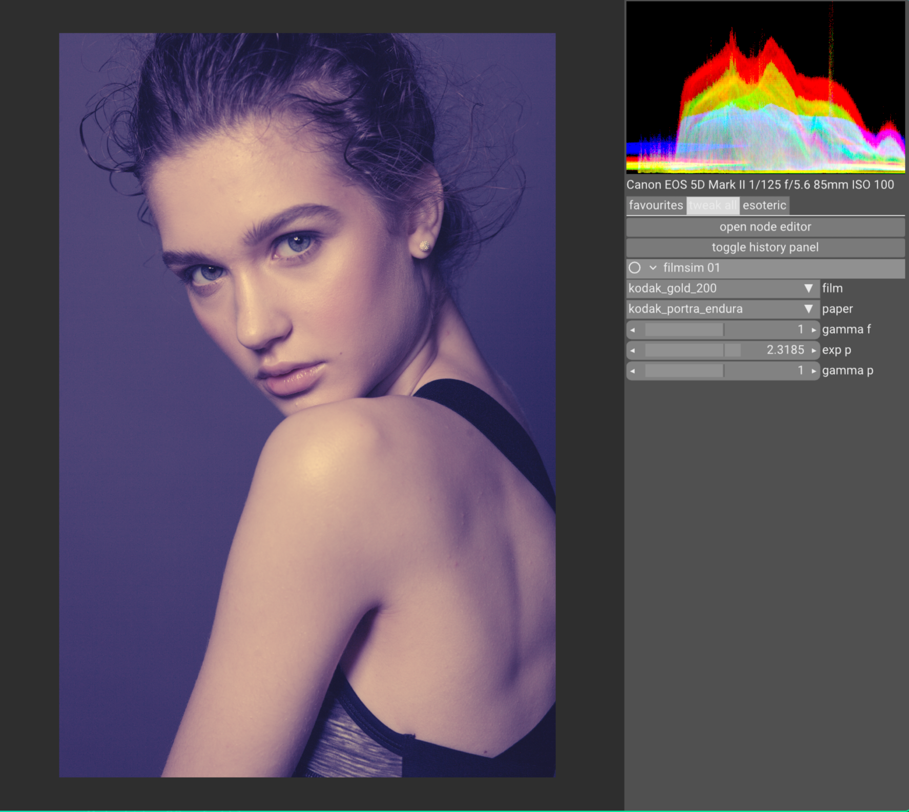
Also I watched you video on film inversion with Nuke, very cool! I am especially intrigued by your decision on using the camera color space without conversion. Indeed it sounds a robust way to avoid any negative values that are not physically possible.

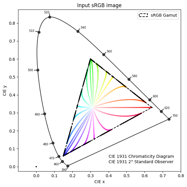
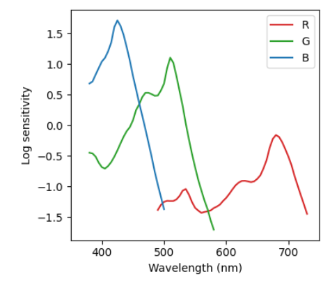
I also notice the cyan explosion in some tests, but still haven’t addressed or pinpointed the root causes. As you demonstrated with your experiment it is most likely relatedto the spectral upsampling of RGB data. From some discussion with @hanatos, I suspect that this is partially related to the fact that upsampling algs are optimized to minimize the errors when XYZ sensitivities are applied. Film negative sensitivities can be quite different from the standard observer. This is for example of Kodak Portra 400:

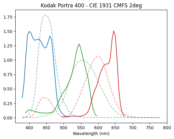
The film absorbs much wider and with less overlapping sensitivities. My reasonng is that upsampled spectra from RGB do not impose good constraints on the region of the spectrum outside XYZ sensitivities. So the generated spectra might have not reasonable values at the edge of the visible spectrum where film absorbs and eyes do not. But I am not the most knowledgeable on the topic to elaborate deeply on it. I will need to spend some more thoughts on this.

This little experiments, even with all it’s limitations, really tickles my brain, and it will trigger some nice thoughts and discussion I think! Thank you for sharing!
I would say that the way we decode the image from the raw, and they way it enters the spectral pipeline has a huge impact.

hanatos · February 22, 2025, 3:08pm

… if i were to bake stuff into images as luts. the profile json, are they all the same shape/wavelength range? i’m thinking i could make one image for say log_sensitivities, where each row would be one film stock. but that would only be a good idea if these are generally all the same and only the data is different.

arctic · February 22, 2025, 3:24pm

All the spectral data are represented on the same wavelength axis (N wavelength data points). Depending on the version 380-780 every 10 nm, or 380-780 every 5 nm. I am keen to stay with the 5 nm representation, that was the optimum that I found early on.

Spectral data are:

film log-sensitivities (log_sensitivity): array Nx3 for RGB layers
dye density absorption spectra (dye_density): array Nx5 for [C,M,Y,minimum density, medium neutral density]
Note: medium neutral density is not really needed. It is only used in the making of the profiles.

There are then density characteristic curves data, all represented on a log-exposure scale (M points), quite oversampled since later I am using linear interpolation on them.

There are:

characteristic curves of the layers (density_curves): Mx3 for RGB channels
characteristic curves of each sub layer (density_curves_layers): Mx3x3 for [log-exposure, sublayer, rgb-layer], used for the multi layer grain synthesis

hanatos · February 23, 2025, 11:31am

thanks for all your explanations! i think i got very many details wrong, and i’m ignoring all the normalisations and illuminants involved in making the image… but i cat at least get recognisable pixels now:

i’m not using any of the 3d luts (maybe i should bake such things), so it’s doing the full spectral upsampling and integration. makes it kinda slow, the full raw resolution processes here in 27ms.

also i had some numerical issues with log10, i think i can just do natural exp/log and scale the lut accordingly.

jandren · February 23, 2025, 12:38pm

A try on how I interpreter those “negative colors” and their purpose a chart:

I see the linear RGB input values as basically 3D coordinates with no real limitation, i.e. we can be anywhere in that space. So we should test that our algorithm is robust for all possible inputs in a reasonably fast way, making sure that those stays black is one way of testing that.

What makes me excited about this spectral stuff is that we can have a better definition of the boundary of valid colors by saying that the spectra has to be positive. In contrast to f.ex. rec-709 (sRGB) primaries that is way smaller than the spectral locus and thus have valid RGB coordinates with negative values in them!

makes it kinda slow, the full raw resolution processes here in 27ms.

I think you can call it slow once you remove that “m” in front of the “s”.

mikae1 · February 23, 2025, 12:53pm

Wait a min… Have you already begun porting the Python code to C? Or is this implemented like in ART?

I agree, that’s blazing fast!

hanatos · February 23, 2025, 1:08pm

heh, i have absolutely no plans for that i want to understand more how the results are formed and which parameters are essential, then implement the grain and preflash etc (left out quite a few things now), and then get into perf optimisation.

and yes, negative rgb is just fine. negative spectral energy is not. the sigmoidal spectral upsampling table i created a few days ago will upsample everything, and it will even be meaningful inside spectral locus. outside it just uses inpainting to give you a positive spectrum close to the coordinate you requested.

glsl. i don’t really speak python and i absolutely hate it if software stacks up toolchains (like shellscript stuff in latex packages…).

mikae1 · February 23, 2025, 1:52pm

Too cool! I hope you’re all prepared for an onslaught of grain loving YouTubers once this gets more accessible.

commutergraphics · February 23, 2025, 2:22pm

this seems really great, I’d been imagining ways to manipulate grain in interesting ways for a while now, it’s not very faithful to film but I’ve been thinking about things like different sizes of grains for different tonal levels doing it with a simulation seems like a possible way to experiment, then maybe do dumb stuff like arrange underlying grains in a perfect grid or different types of random patterns etc, stuff that couldn’t be done with film, maybe that would be something like masking areas in darktable then applying different instances of this to it, frankensteins film, velvia in the skies and astia for the birds

arctic · February 23, 2025, 5:35pm

27 ms, thats crazy! I think that the “camera” 3D LUT and the “scanner” 3D LUT could be backed. I am not sure about the “enlarger” one, since the color balancing with CMY filters is changing the LUT, and this is one of the main controls.

The fact that you can see at the end of the pipeline is already something!

Thanks for the comment, it makes sense. Negative ACES2065-1 values are for sure outside of the visible locus, so I guess it is kind of an extreme region to test computations on visible images, but with spectral processing maybe it has more meaning.

hanatos · February 23, 2025, 6:32pm

… i can not for my life get neutral renditions out of this:

this is with enlarger filters set to 0.005,0.008,1…

are there any obvious places where overall colour balance would be thrown off? oh, and this lamp, does it have a base spectrum on its own? now i’m just mixing the thorlabs filters…

i’m also not using any of the D50 or D55 illuminants… but i figured illuminant E is not too far off.

arctic · February 23, 2025, 6:33pm

I implemented and tested a bit the method of spectral upsampling by @hanatos. It is available in the large-color-space branch of agx-emulsion, I will move it to the main after some more testing.

I have some preliminary qualitative results (using raw files from signatureedits.com). I think overall there is an effect on the saturated colors. The new method from hanatos (called here hanatos2025) can produce spectra for any tristimulus value in the visible locus. I think it is great for it’s simplicity and results. The old method called mallett2019 is only valid tor sRGB, so it transforms and clips the values to sRGB before the spectral upsampling.

I exported some test raw images in linear Rec2020 and run some simulations.
Here are a few comparisons, in which I changed only the upsampling method keeping all the other parameters unchanged (unless stated).

(left) hanatos2025 and (right) mallett2019, Kodak Portra 400 and Portra Endura

As a side note, I added also a band pass filter to the virtual camera (filtering near UV below 400 nm and above 680 nm). The most problematic point was that some stocks like Portra 400 have a very blue/near UV absorption and the upsampling methods really do not limit what happens when XYZ sensitivities goes to zero.
The filter look like this:

In blue is shown the sum of the standard observer XYZ sensitivities. The band pass cuts the part of the spectra that cannot be constrained by the upsampling methods (that optimized for minimum XYZ error).

I already noticed from the beginning of the project that reds in portra were quite pink compared to other stocks. Now they behave in a more reasonable way.
(left) hanatos2025 with filter and (right) hanatos2025 without filter, Kodak Portra 400 and Portra Endura

I compensated the image without bandpass filter (-15Y) to balance a bit the warmth.

(left) hanatos2025 and (right) mallett2019, Kodak Portra 400 and Portra Endura

The crop of the background shows that hanatos2025 is more smooth in the high saturation yellow flowers, retaining the smooth color transition to the center of the flowers.

(left) hanatos2025 and (right) mallett2019, Kodak Gold 200 and Portra Endura

In this portrait, hanatos2025 retains some more saturation, and I think the transition with the out of focus edge of the hair is more pleasing. The image seams also to have more “depth”.

(left) hanatos2025 and (right) mallett2019, Kodak Gold 200 and Portra Endura

Some special colors are definitely more affected than others, like lime-greens.

I did also some quick test with this stress test image that explore the edges of a color space and the desaturation paths. This stress test image already presented earlier in the thread.

This is when I imported the image as sRGB with cctf decoding active.
(left) hanatos2025 and (right) mallett2019, Kodak Portra 400 and Portra Endura

By bumping exposure 2 stops and 0.25 print exposure we can reveal the “cyan catastrophy”, also noticed by @liam_collod in his tests. The new method seams a bit worse at it.

(left) hanatos2025 and (right) mallett2019, Kodak Portra 400 and Portra Endura

We can also import the image as if it was linear Rec2020, and explore the edge of the Rec2020 color space.

(left) hanatos2025 and (right) mallett2019, Kodak Portra 400 and Portra Endura

0 stops, 1.0 print esposure

+2 stops, 0.25 print exposure

There are some issue with the very blue corner of Rec2020 with hanatos2025, and the sRGB clipping of mallett2019 is super clear. The performance on the large color space are clearly much better for hanatos2025 with no surprises here.

arctic · February 23, 2025, 6:45pm

This has been a huge struggle also for me, for quite a long time. I have seen all the possible weird colors.

Color enlargers uses tungsten bulbs (approx. 3200K), and sensitivities of print paper are balanced for it, i.e. they have stronger blue sensitivity compared to red. In the simulation I am using a black body emission spectrum at 3200K.
This is Kodak Portra Endura sensitivities as an example.

Right now I am always keeping fixed the cyan filter at 0.35 (in a 0-1 range), and on average the yellow filter is 0.6-0.8 and the magenta filter 0.4-0.6. The value used in the python package are in the .json of fitted neutral filters in agx_emulsion/data/profiles.
Also in the real darkroom workflow, the C filter should not be touched and only Y and M filters should be used.

This is probably true, I just used them as the one recommended for viewing the prints (D50, used to compute the final XYZ >> RGB for viewing the print) and for the neutral density measurements by kodak (D55). But not used in the sim otherwise (or better mallett2019 used them).

hanatos · February 23, 2025, 6:52pm

hm could this be the case where the spectral peak is way narrower than the 5nm spacing used for integration? that might explain the sharp drop in brightness for some shape of blue. i suppose since we know where the peak is we could devise specialised quadrature rules/monte carlo importance sampling.

arctic · February 23, 2025, 7:05pm

I ended up computing the spectra with a 1 nm resolution (should be enough right?), blurring them with 2.5 nm sigma gaussian kernel (approx 6 nm FWHM), and resampling them at 5 nm step. Still the issue might be present. I can try to blur them more and see if the drop in brightness improves.

Edit:
This is with spectra computed with 0.5 nm step and blurred with a 10 nm sigma, then resampled at 5 nm step.

hanatos · February 24, 2025, 7:55am

hmm okay thanks. so you’re saying it just looks like that. these gradient images are generated how? probably some hsv bs and then converted to rgb and that simply reinterpreted as rec2020… nobody says this is smooth to begin with.

arctic · February 24, 2025, 8:52am

Even worse, just some arbitrary ramps over the edge of the color space. The bottom part of the “stress test image” is made by scaling the RGB plot below from 0 to 1.
Indeed I don’t like it much. I have just seen them around (in not scientific settings) when comparing film sim. So I agree that this is a bit of a dumb qualitative comparison.

CIECAM16 lightness looks pretty spiky, so the discontinuity should be expected. I got to find better ways.

Also the interplay of the spectra with sensitivities and the later part of the film sim pipe might not be straightforward.

hanatos · February 24, 2025, 12:15pm

some more detailed questions:

density_cmy is 3 channels per pixel and holds c,m,y as the name suggests, and in this order? because the order on the lamp filters is ymc.
how do i get density_cmy? by doing a per-channel lookup of log_raw (rgb) through the density_curves lut? like log_raw.r → density_curves.r → density_cmy.r?
how do i get spectral density from density_cmy and the dye densities? dye_density is three spectral quantities, so i multiply density_cmy.r to dye_density.r[wavelength], do that for r,g,b and sum the three spectra? (and then add the min density/fourth channel times some constant regardless of density_cmy)
the filters are transmittance filters, right? so i blend in the “strength” of the filter by mixing it with a constant 1.0 spectrum, and then multiply all three spectral filters (for c,m,y).

PhotoPhysicsGuy · February 24, 2025, 12:58pm

It’s the outer surface of whatever RGB cube you have. Cube corners and edges aren’t smooth (trivial), but the cube-faces are as smooth as can be.
That cyan behaves different than yellow is the oddity, imho.

(In testing LUTs or DRTs the cube-faces should at least stay smooth and don’t get more kinks. In addition the gamut edges and corners could be translated into smooth edges/corners as well. Channel crosstalk would smooth out edges for example. It’s a stress test because it samples the input-RGB basis-vectors and their mixtures. If the output of that is smooth, things closer to the [0,0,0] to [1,1,1] axis probably behave as well, except for really broken LUTs. )

arctic · February 24, 2025, 2:57pm

The order CMY (analogously to RGB) is correct for the variable density_cmy and used everywhere except enlarger filters. The choice of having the fitted neutral filters as YMC came from studying physical enlargers datasheet, I read some stuff from Durst for example.

In the physical devices from Durst and their manuals, the order of the filters is usually YMC. Y roughly controls temperature and M tint. It is probably an unhappy choice for the code.

Yes!
I compute raw as the product of the irradiance spectra and the sensitivities, then integrate over the wavelengths.

raw  = contract('ijk,km->ijm', spectra, sensitivity)

I make sure that raw is normalized such that whatever i think should be midgray in the image has value 1 (normalizing only by the green channel). And apply exposure.

illuminant = spectra_lut[-1,-1,-1] # spectrum for input linear RGB=[1,1,1]
raw_midgray  = np.einsum('k,km->m', illuminant*0.184, sensitivity) # use 0.184 as midgray reference
raw /= raw_midgray[1]

raw *= 2**exposure_ev

Then I do a linear interpolation of density_curves (again RGB/CMY ordering), that is represented on the x axis variable log_exposure, both in the json, with the log_raw data computed (log10(raw)).

That sounds correct!
density_cmy multiplies dye_density spectra channel wise. And the fourth column dye_density[:,3] is the density minimum, and it is summed.

def compute_density_spectral(profile, density_cmy):
    density_spectral = contract('ijk, lk->ijl', density_cmy, profile.data.dye_density[:, 0:3])
    density_spectral += profile.data.dye_density[:, 3] * profile.data.tune.dye_density_min_factor
    return density_spectral

In this snippet: ij are the pixel of the image, k is the CMY channel, l is the wavelegth.

Filters are in transmittance, and taken from Thorlabs datasheets (only the CMY ones):

In my code I blend the filters and apply them to a 3200K black body illuminant with this code:

dimmed_filters = 1 - (1-filters)*ymc_filter_values # following durst 605 wheels values, with 170 max
total_filter = np.prod(dimmed_filters, axis=1)
filtered_illuminant = illuminant*total_filter

here filters is an array [wavelenghts, ymc_channels], and ymc_filter_values a 1D array with the three filter values in a 0-1 range.