Hello, problem opening files on Xubuntu 24.04 with 8GB RAM (too low on RAM perhaps?).
I followed the installation instructions on Github, using conda. Everything installs fine and the program starts. But when I drag a photo on the application, nothing opens/happens. Instead there are error messages in the console.
(agx-emulsion) paul@graveyron:~/apps/agx-emulsion$ python agx_emulsion/gui/main.py
MESA-LOADER: failed to open nouveau: /usr/lib/dri/nouveau_dri.so: kan gedeeld objectbestand niet openen: Bestand of map bestaat niet (search paths /usr/lib/x86_64-linux-gnu/dri:\$${ORIGIN}/dri:/usr/lib/dri, suffix _dri)
failed to load driver: nouveau
MESA-LOADER: failed to open nouveau: /usr/lib/dri/nouveau_dri.so: kan gedeeld objectbestand niet openen: Bestand of map bestaat niet (search paths /usr/lib/x86_64-linux-gnu/dri:\$${ORIGIN}/dri:/usr/lib/dri, suffix _dri)
failed to load driver: nouveau
MESA-LOADER: failed to open swrast: /usr/lib/dri/swrast_dri.so: kan gedeeld objectbestand niet openen: Bestand of map bestaat niet (search paths /usr/lib/x86_64-linux-gnu/dri:\$${ORIGIN}/dri:/usr/lib/dri, suffix _dri)
/home/paul/apps/agx-emulsion/agx_emulsion/gui/main.py:24: FutureWarning: Public access to Window.qt_viewer is deprecated and will be removed in
v0.6.0. It is considered an "implementation detail" of the napari
application, not part of the napari viewer model. If your use case
requires access to qt_viewer, please open an issue to discuss.
  layer_list = viewer.window.qt_viewer.dockLayerList
WARNING: QOpenGLWidget: Failed to create context
WARNING: QOpenGLWidget: Failed to create context
WARNING: composeAndFlush: QOpenGLContext creation failed
WARNING: composeAndFlush: makeCurrent() failed
WARNING: composeAndFlush: makeCurrent() failed
WARNING: composeAndFlush: makeCurrent() failed
Here the program hangs.
Seems that the nouveau driver can’t be found. On my system it is not in /usr/lib/dri (that folder does not exist). A locate nouveau shows the following: /usr/lib/xorg/modules/drivers/nouveau_drv.so.
I haven’t tried Dehancer (or Filmbox), just admired the gorgeous examples they have on the website and some videos on Youtube. Since they want to run on video, I guess they have different priorities for overall computational efficiency. I think the simulation in agx-emulsion is not true because it is not based on real profiled scans. There is a lot of reasonable guessing. At the same time it is a physically based model end to end, so it might be more “robust” and “smooth” in more edge conditions, i.e. it might fail more smoothly.
I was thinking of adding a “tint” control for the toe region of the negative, this should add some flexibility for toning the shadows independently. Also it should be able to control the color of very underexposed negatives, that can change quite a lot (just looking at example online) and I guess depends from the development conditions. It’s in my todo list.
That’s a good question. At the beginning I was always correcting the white balance with darktable. Recently I started fixing the white balance at 5500K and I do like the results, e.g. sunset shots for example that I tend to leave warmer in this way. I haven’t done a serious comparison, but I suspect that subtle differences should be present due to the crosstalk in the enlarger filtering and paper absorptions (not precise as the digital wb). Plus it sounds more correct.
Kodak and Fuji apparently are balanced for 5500K and 6500K respectively. I don’t have a good reference to support that, but this is what I am using in the spectral up-sampling from sRGB. The algorithm from [Mallett2019] should work very well only for 6500K and just ok for 5500K, not well for lower temperatures. Tungsten balanced film will have to wait a better up-sampling alg implementation. I still tend to use 5500K as a default wb for the input.
Thanks! That thread is impressively stimulating to scroll, there is so much nice visualization and color science at play. I am kind of shocked I will have a read.
Having images that can show problems would be great! I am pretty sure we will find many issues. I will look for those images, but of course, I will be happy to be pointed to the repo if you know where to find them @ChrisB.
It looks like a GPU driver problem that should be independent from agx-emusion (that does not use GPU). napari is gpu-accellerated as far as i know. Try to run napari independently, from the terminal run this:
> conda activate agx-emulsion
> napari
And try to load the same image. If you have the same problem I am afraid I am not the most knowledgeable person to find a solution for this. Maybe write me a direct message if you have more info, so we leave this thread more free for discussions.
About the ACES 2.0 thread (CAM DRT), I would “take it” carefully. The use of Color Appearance Model in image formation is highly debatable to say the least.
Thank you for the links! I’ll experiment with them. They are going to be useful, since I will expand the input color space to larger ones.
Nice Lego render. Do you think the Lego figurine in the background has some red gradient issues? Or is this image used to reveal anything in particular?
about that where would that have to happen? my current understanding of the code is that it would be one of the first steps of the film code, where the input image is converted to linear light rgb and then passed through the density look up table to give cmy densities. i think this is the profile that is precomputed in the longish json files… (i think i want these as a lookup texture) how/where do you compute it? i’m assuming internally it has a linear rgb → spectrum → density of turned grains pipeline?
i would probably just use a simple full-gamut sigmoid emission upsampling method for rgb to spectrum out of srgb. this requires a simple 2D lut from xy chromaticity to coefficients for the parametric spectra (can provide lut). some more broken/matrix-based input device transforms would give you rgb values for the input image that are even way out of spectral locus. i’ve seen some of that in the aces thread. we can’t upsample these coordinates, they’ll need to be clamped to real stimuli first (don’t want negative energies on some wavelengths).
Right now, I am optimizing the pipeline to make it more clear and efficient. If anything looks stupid please don’t hesitate to say that.
I confined all the spectral calculations in three LUTs (3D LUT 1, 2, and 3).
I can now compute 100MP images without running out of RAM! Still ages to compute.
(sorry the huge image, I compressed a lot though)
And thank you @Artaga734 for helping with some profiling of the code!
I am attaching a small scheme of the pipeline that might make things more clear than my dirty code. I specified input-outputs of the LUTs. All variables are 3 channel images.
You can clearly see the two step of the imaging system (film + print). The 3D LUTs are covering the spectral calculations happening in the camera, enlarger, and scanner (or I guess more precisely in our eyes). I think that some magic happens in 3D LUT2 and 3D LUT3 where there is subtle crosstalk among the channels and the spectral density saturates smoothly, slowing eating away the light around the absorption peaks of the dyes.
Exactly! It is going to be at the very beginning of the pipeline. I am converting input image >> linear rgb >> spectral upsampling x film sensitivities >> exposure of each layer of the film (3 channels).
And you are right that 3D LUT1 could become 2D using only xy chromaticities. I didn’t think about that! Is this a standard way of doing things?
That would be great actually! I don’t know the “full-gamut sigmoid emission upsampling” method, do you have a reference? And is this what you would recommend for best quality results? I was also playing a bit with colour.recovery.LUT3D_Jakob2019 to precompute spectra in a 3D LUT to be stored and used in 3D LUT1 (this is still yours , I glanced the paper and it is an amazing piece of work). Do you think that it is an overkill solution?
Also I noticed that in Jakobs2019 the spectra can change quite a lot at extreme values of lightness (10^-4 and close to 1). For example I was calculating the spectra for al the possible values of the ACES2065-1 space in a grid 32x32x32 (that might be dumb). I was limiting the values between 0 and 0.1 in 32 steps. I restricted to 0.1 because values closer to 1 were broadening quite a lot the narrower spectra. Is this a limitation of the method or somehow intended?
(TL;DR: just a huge thanks from me too! For more, keep reading at your own risk
Hi,
I just wanted to join the crowd of fans of this awesome project. I have been playing with it for the past 10 days, essentially since the moment it was announced. I am continuously amazed by how easy it is to get great results. Kudos @arctic!
So, I immediately started thinking about how to incorporate this into my workflow. The code is way too complex to just “borrow/steal” it, and it requires a level of knowledge of the whole film processing pipeline that I simply do not have (though the diagram above helps quite a lot in getting the big picture).
At first, I tried to see whether I could match the renderings with more conventional digital tools for tonemapping and colour grading. Well, yes, you can get close, but it’s quite a bit of work, and the closer you get, the more fragile the “standard digital” way becomes (meaning: you might get close for a particular picture, but getting something robust seems much harder).
Therefore, I started thinking of another way, and I now have something that I consider good enough for my purposes. Basically, I managed to extend ART’s support for 3dLUT plugins to allow it to use “externally computed 3dLUTs”, that can run arbitrary code to compute a LUT in CLF format, and then use it in the ART pipeline. After a bit of boilerplate (really, just a couple of hours of coding), I managed to get something working. I can now enjoy the awesomeness of @arctic’s work (*) inside ART – and this makes me smile
Here’s a little demo just to prove I’m not making things up:
(As you can see, it takes some time to (re)compute the LUT after changing settings, but (a) this is cached so reapplying the same settings is then fast, and (b) my laptop is really getting old now…)
(*) NOTE: this only works for the “tone mapping” part of AgX-emulsion; I had to turn off all the spatial processing (e.g. grain, halation, and other diffusion-based processes). This is not a big deal for me, since I was mostly interested in the tonemapping stuff, and ART has some (way less accurate and convincing, but still) other way of faking grain and halation. But definitely something to keep in mind.
awesome, thanks for the schematic, that helps a lot indeed! initially i thought i’d have to store spectral frame buffers as intermediates and was thinking of ways to compress them, but that doesn’t seem to be the case, so that’s great. about the spectral upsampling stuff:
no, usually we do 3D, because there is a joint limit on how saturated and how bright a reflectance spectrum can be (mac adams limit, can’t reflect more than 100% in each wavelength, so more colourfulness means less reflectance/darker). this means the spectral shape has more freedom for darker reflectances and it’s important to include that in an upsampling algorithm.
now we’re dealing with emission i.e. unbounded signals here, not reflectances.
by “full gamut sigmoid emission upsampling” i meant [Jakob 2019] (the sigmoid part), but with a lut that spans the whole spectral locus (full gamut). also it should be for emission, not for reflectances. this is not a natural match to bounded sigmoids, but we can always scale the overall energy up, keeping the shape. what i’ve done in the past is use a 2D table on xy chromaticities (or something similar directly in 2d/rec2020 because that’s my working space), and do sigmoid upsampling at some medium brightness, and then scale the spectrum up to match the energy of the input signal.
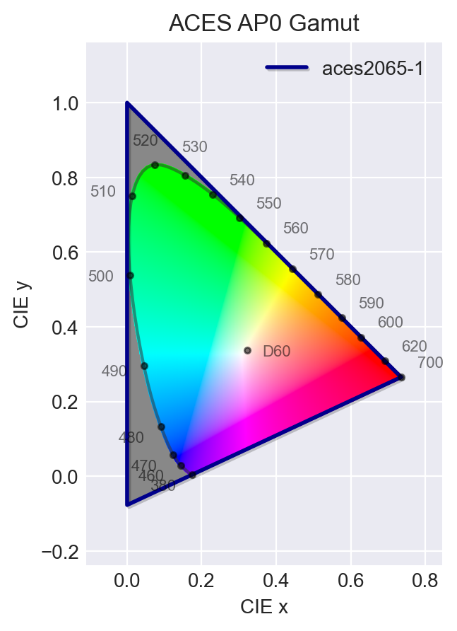
how did you do this? does the colour code only read the precomputed coef files or run the gauss/newton optimiser? the sigmoidal function class here can represent spectra pretty much all the way to the end… but that’s the end of the spectral locus/mac adams limit. ACES AP0/2065-1 is pretty much XYZ with the red corner cut off for better looks: https://facelessuser.github.io/coloraide/images/aces2065-1.png
that means there are some values outside spectral locus that require imaginary stimuli/don’t have a valid spectral power distribution as representation. maybe you ran into this region?
Hey @agriggio! Really appreciate this message and your work. That was very fast! I like how you distilled the essentials in the GUI, with all the basics needed for the tonemapping. Great job!
I am also in a way learning from the output of the simulations. It is shaping my tastes, and looking back at images I processed before, it showed me that sometimes I should dare more with contrast and saturations (but in the right “ways”), and the simulation is selecting the right colors palettes that do this comfortably. I guess that investigating how the LUTs are actually shaping the colors might give some general insight, to develop generic and efficient tools that mimics the simulations output.
My interest in grain simulations was my gateway into this project, but this makes also total sense.
As a side note, I think that to be more true to the analog film+printing system, I would change the print gamma and keep the film gamma untouched if possible. This makes also more sense because of how DIR couplers works based on the density values in the film.
Indeed that makes a lot of sense, thanks for the clarification!
The colour package can do both. Recall the LUT of precomputed coefficients from the supplementary of [Jakob2019], run the optimizer (with a much greater computational cost), or also compute a new LUT if needed. I was definitely comparing spectra in the imaginary region. This is what I had, exactly on the edge beyond the green side of the visual locus.
Hi @arctic
I just wanted to chime in as well and say really nice work on this project. I’ve been tinkering with it and am really impressed and intrigued with the approach.
Expanding on @ChrisB’s reply above, I was wondering if you had any interest in adding exr as an input image format? In addition to being a generally terrible image format, png is really not designed to encode “scene-referred” pixel data. Multiplying down a “scene-linear” image and encoding it as a 16 bit linear exr is incredibly inefficient and poor quality due to the way the quantization works (16 bits distributed linearly over a 0-1 range on a multiplied down “scene-linear” image will put most of the image data in the lowest region, resulting in fewer bits of precision to encode the data). Another workaround might be to add some “scene-referred” transfer functions to encode the image data in a log encoding and store that as a 16 bit png. But now that openimageio is available as a python wheel and installable with uv / pip, maybe it’s worth investigating exr support?
Happy to help if I can when I get some spare time!
Again, thanks for the great work, excited to play with this more.
Hey @jedsmith, I am glad you manage to play with it! Thank you for the comment.
Listening also to the feedback from @ChrisB and @liam_collod, I just added to the main branch a few updates, including the possibility to load exr files (32bit and 16bit). I am using now OpenImageIO as recomended, and I dropped the need of downloading the freeimage backend. I quickly tested and seems to work fine, but if you test with more exr files let me know how it goes.
The main branch has now also a few optimization for accelerating the grain synthesis with some numba functions, and all the spectral calculations are now behind 3D luts. The memory bottlenecks should also be drastically reduced.
I updated the requirements with the new packages. I had to revert to a slightly older version of numpy for compatibility with numba.
The input color space can also be different than sRGB, but it will be internally converted to sRGB and clipped at the very beginning of the pipeline to use [Mallett2019] spectral upsampling. The color space must be selected in the input tab. Larger spaces are coming (WIP).
Nice then I don’t need to make a PR with my .exr implementation that I did this morning!
Definitely a workflow improvement to use linear .exr files, makes it possible to adjust the exposure in darktable with sigmoid activated and then just deactivate at time of export. Just load and deactivate “input/apply cctf encoding”, no auto exposure required!
I have to confess as being one of the pure tone mapping users atm but that is really interesting enough. Can’t really say much about the correctness of it all at this point more than that it looks good and that I love the first principles approach. Looking forward to digging deeper into this, especially wider gamut inputs and how that handle later.
I love charts as a complement to images so here is the result using the syntheticChart.01 from ACES.
kodak_gold_200 + kodak_endura_premier
No auto exposure/compensation or other variations from defaults other than disabling all spacial effects and grain.
The horizontal bars in the middle are zero at the center and negative towards the right so something goes wrong with “negative” colors.
Some colors that desaturates later but not as bad as normal per-channel methods would do if you just clipped the gamuts to their boarders.
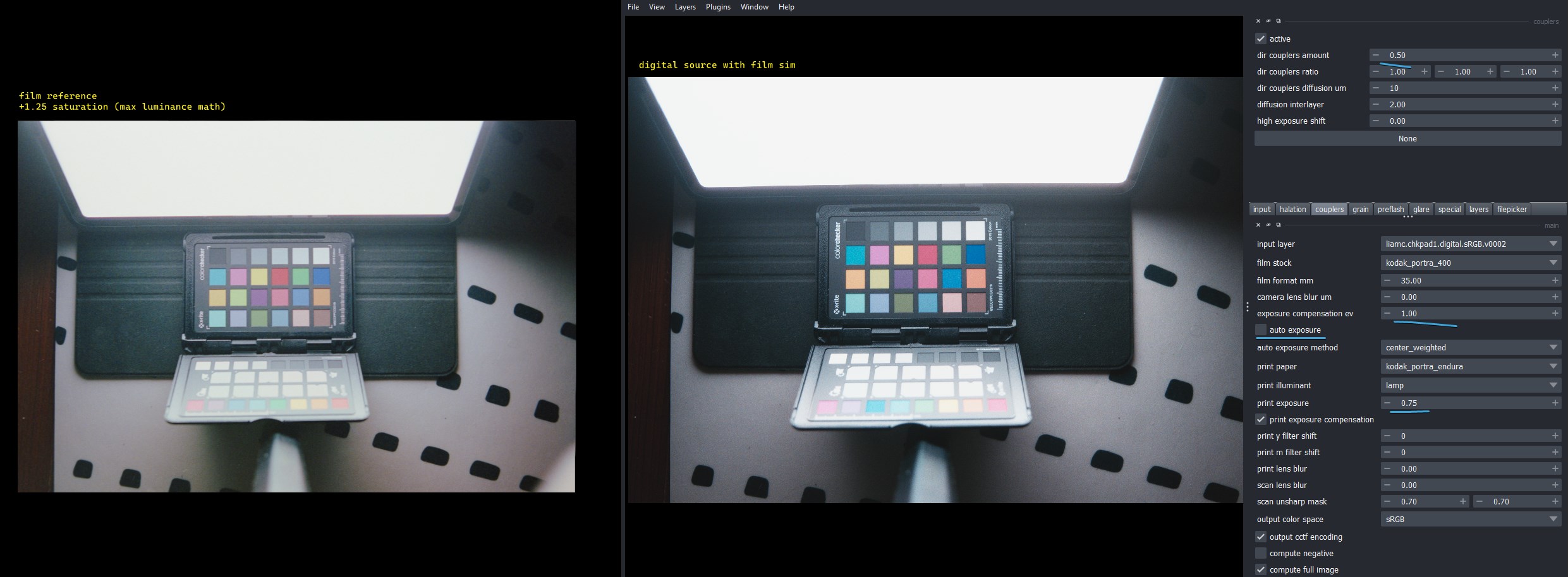
left is the film ref that have been subjectively tweaked and generated using my personal film scanning workflow; note I had to increase the saturation on the film ref by +1.25 using “max luminance math” as it was pretty bland and hard to compare with the sim.
right is the result of the sim using the digital source images with sRGB primaries (I reconverted the provided BT.2020 exr to be safe). I reduced the dir couplers again to try to match the saturation of the film ref.
So there is a lot of bias and issues in that comparison but straightaway I think I can notice the bottom cyan patch to completely explode which is very interesting.
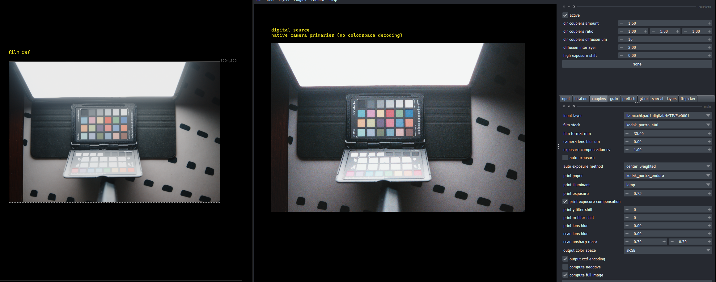
As this patch issue rings a bell I decided to run a second test:
same ref on the left (EDIT: please ignore left image, it’s the digital with an arbitrary image formation, use ref on previous picture sry)
on the right I I now used the digital source that have been debayered to the native camera colorspace instead (file not provided, I did it on my side), and then just interpreted as sRGB in the film-sim app; basically skipping all colourimetric transformations. To compensate I had to increase the dir couplers amount this time.
Now we can see that the blue patch doesn’t explode anymore and the overall tones feels closer to the film ref.
I can’t conclude much with that little experiment but to raise the issue that source image encoding and decoding also seems to play an important role to get the whole image formation pipeline closer to analogue film.
hmm i think 32 cubed might not be super high res… maybe the discretisation near the edge changes the result a lot. another thing to consider is the limits of the gamut. these bounded spectra fall inside MacAdams limit, i.e. can’t go to negative energies (outside spectral locus, sideways) and can’t be too bright (reflectances are <=100%). i think in the huge AP0 gamut you’d encounter both limits. the optimiser may or may not diverge in such cases.
but yes, see pm for special cased upsampling code, hope to see it upstream soon
Indeed, I also am afraid that true film simulation of the output of real film stock is probably impossible just with first principle. Some kind of real reference is necessary to understand better. Maybe one could think to fit part of the model to some real data. I think it is better to say that the output is somehow inspired by a film-stock/print-paper data within the limit of the model.
I don’t get much this part about the negative colors. I found this page where they describe the rationale of this test image. But what do the negative colors should show about the tone mapping pipeline?


