Yes, there are good data available, the datasheet looks of good quality with all the necessary data. I agree that print film would be very interesting to try. This already came up in a discussion with @PhotoPhysicsGuy. I added it on the future list of the film stock to profile.
3 Likes
I think it’d be interesting to create a virtual Fuji Frontier scanner model somehow if possible. Then that can maybe be used along with real world tests/scans to validate the results and simulation of film stocks. I believe that’s what VSCO ended up creating. It’s been written about a little bit here:
- VSCO Film X & The Imaging Lab | VSCO Engineering
- How VSCO Builds Film-Like Smartphone Photo Filters in Its Lab | WIRED
- Inside VSCO’s Imaging Lab : App Store Story
Here are some patents related to the Fuji Frontier. The first link I believe has a graph with the wavelength LEDs used.
- US20010026369A1 - Light source device and device for reading original - Google Patents
- US20030081211A1 - Light source device and image reading apparatus - Google Patents
- US6751349B2 - Image processing system - Google Patents
- US6067109A - Image reading method - Google Patents
- US6791721B1 - Image reading device - Google Patents
- US6665434B1 - Device, method, and recordium for correcting color imbalance of an image - Google Patents
- US4893178A - Simulator for automatic photographic printing apparatus including inversion circuitry and spectral characteristic compensation - Google Patents
4 Likes
Reading this gave me a new level of respect for VSCO. They must have a lot of fun with all this characterizations.
Thank you for searching the patent literature.
Having the LED light source spectra is a good start. I guess the most difficult part will be to understand what is the actual data processing pipeline from their RAW scanned file (calibrations/transform matrices/curves… etc). VSCO (and negative lab pro) might solve this by profiling input/output of the scanner with color test charts.
If we find any decent complete source with the methods behind the scanner processing we could attempt something from first principle. I bet it is going to be very hard to find it, though.
I am skimming the patents for hints.
1 Like
I have a preliminary first test using Kodak Vision Premier color print film 2393.
I am struggling fitting print filters using my enlarger light source (I will have to change it compared to what RA-4 paper uses, or trying to understand the issue).
The comparison uses Kodak Ultramax 400, that by chance can be fitted.
(left) Kodak 2393, (right) Kodak Portra Endura
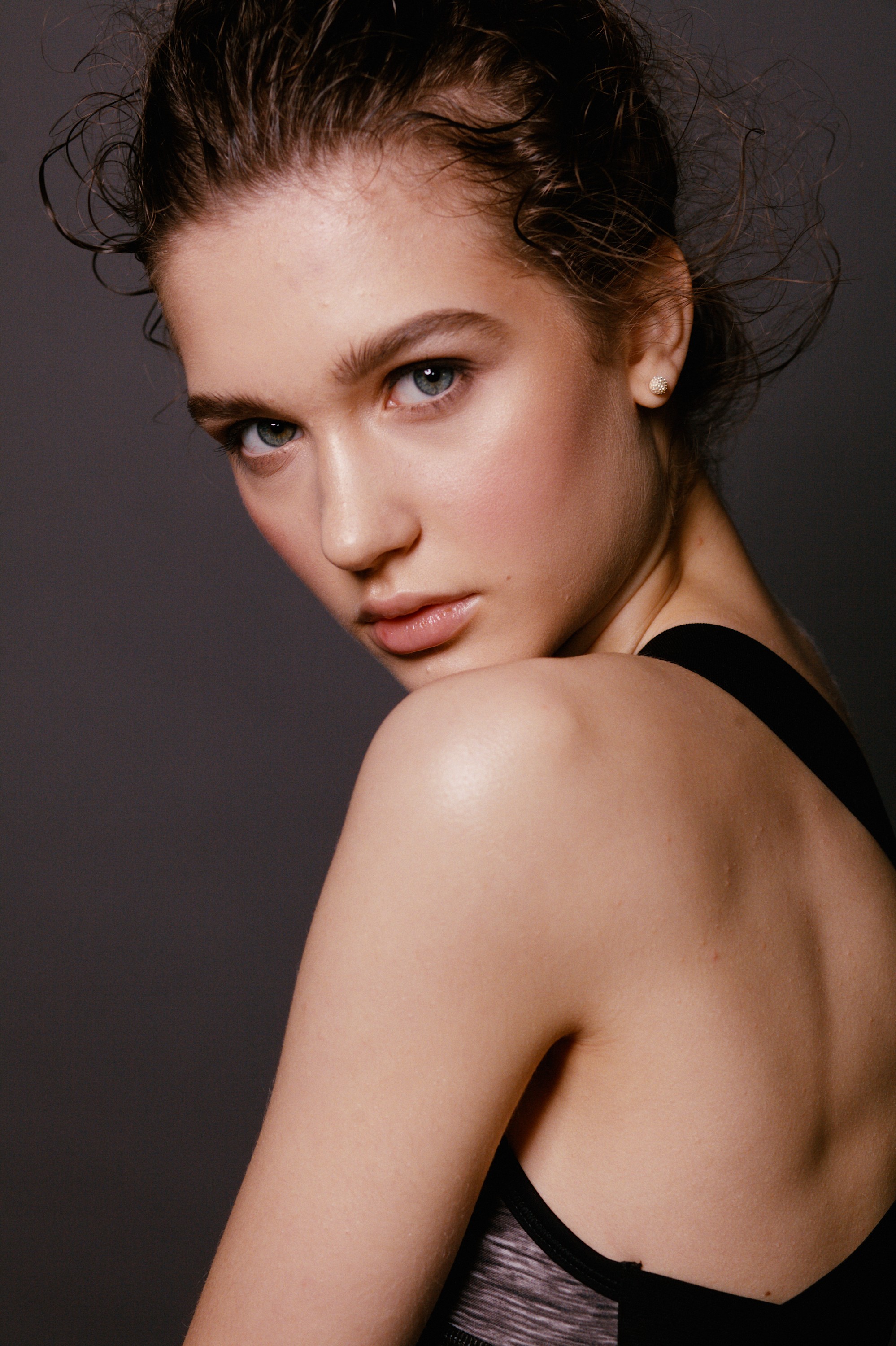
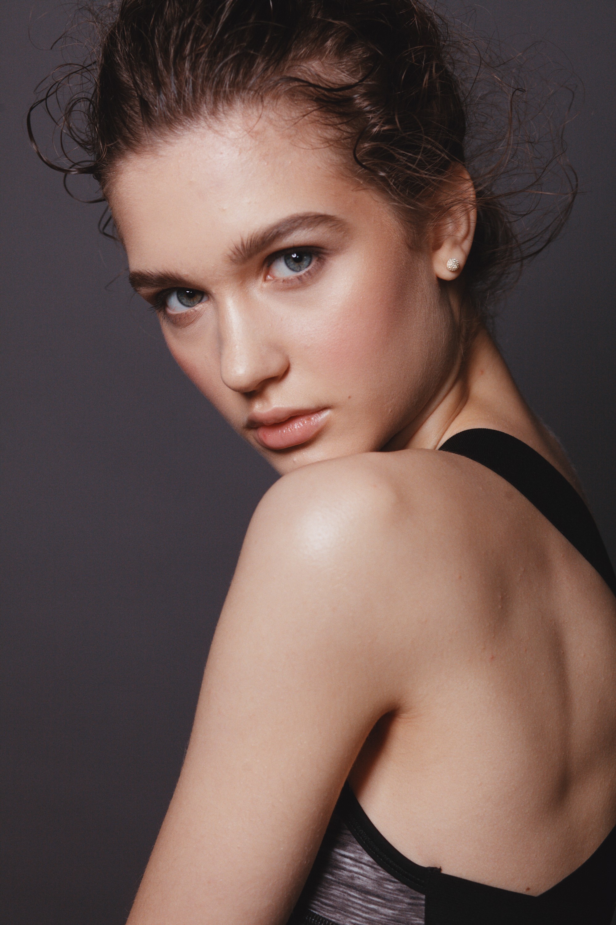
I notice very deep blacks. Density curves reach almost 6 OD!
I am not sure if we should mix photography film with movie print film. It might be an heretic thing to do.  But this is what we got for a first test.
6 Likes
I had no idea they were this serious about film simulations. I always had them pegged as a simple preset app, but this gave me a lot more respect for their work!
1 Like
just wanted to mention here that i had some issues with very saturated/narrow spectra: Problem with filmsim artifacts · Issue #164 · hanatos/vkdt · GitHub and share a new upsampling lut. i know agx-emulsion uses dense sampling and some regularisation for better integration, so there might not be any problem. i now use a lut for the spectral upsampling that stops creating narrower peaks just before it reaches the boundary of the spectral locus. as a result the inpainting for non-physical stimuli are also much smoother:
spectra-em.lut (4.0 MB)
2 Likes
Not sure if this will be helpful or not, but when I was looking into film scanning a while back I came across this Kodak patent for a bandpass filter that can be used to remove problematic portions of the spectrum to make different scanner light sources behave more similarly. Maybe adding this filter will smooth out some of the fitting issues you’ve been having?
Kodak_Printing_Filter_Patent.pdf (682.1 KB)
1 Like
My idea with my proposed test image was to see how the spectral upsampling behaved when reaching the spectral boundary. I will try to make some tests myself and see if I can provide some insights. The new results using hanatos large gamut spectral upsampling method does work a lot better so its all very promising!
I also realized that another test source could be actual hyperspectral images! Here are some reasonable sources I found so far.
-
Multispectral Image Database from Columbia Imaging and Vision Laboratory, a small but promising selection of images. CAVE
-
Large Hyperspectral imaging dataset from Bian Lab in China, requires request for access which I haven’t tried but seems like it should work. GitHub - bianlab/Hyperspectral-imaging-dataset
-
A dataset from Havard, lower quality: Statistics of Real-World Hyperspectral Images
-
Lower quality and resolution dataset captured with a rotating line camera: danaroth/icvl · Datasets at Hugging Face just git clone the link to download.
-
Dataset of faces, again requires request for access which I haven’t tried myself. But faces are of course of interest! GitHub - hyperspectral-skin/Hyper-Skin-2023: Introducing Hyper-Skin data with 2 types of data pairs: 1. (RGB, VIS), 2. (MSI, NIR)
-
Finally one that looks very promising and says it should be open but I haven’t been able to access. Adding it here if anyone else manages access it: GitHub - boazarad/ARAD_1K: ARAD_1K Spectral Image Dataset
I also know a local company in Umeå which works with hyperspectral images. I might be able to ask them to take a picture or two with one of their cameras if you have anything specific and doable you had loved to have a hyperspectral test picture of.
5 Likes
Ha just a side note we had a student just do a visit with us from the university there. She stayed for a couple of weeks here in Canada. She did a little background on the area and the university in her talk. That looks like a lovely part of the world… 
Looks very nice! Kind of relates to one question I have. I send some pictures for print on Fuji Crystal Archive paper. For these pictures I guess it’d make sense to disable the paper simulation part of agx-emulsion or else they’d be “double papered” with very washed out blacks.
For the files that should be viewed on a screen (uploaded to my website or social media) I’d like to have the paper sim enabled.
Would this even be possible (and is my thinking right)?
EDIT: Perhaps one way to go at it would be to assume that I had scanned a paper print. After scanning a paper print in the darkroom days I’d of course set black and white points. Would it be able to provide black and white point controls as a last step in the process in agx-emulsion?
But yeah, I’d still “apply” the “color characteristics” of print paper twice?
I should perhaps also add that I really appreciate agx-emulsion’s inclusion of the paper characteristics. Most other film simulation solutions I’ve come across try to to emulate the color characteristics of a scanner (usually Frontier or Noritsu). Negative film, however, was never meant to be scanned, it was meant to be printed.
Thanks @hanatos for the updated lut and sharing the GitHub issue!
I replaced the old one.
Indeed, just looking at the coefficients maps, they look way smoother past the spectral locus.

I compared the old LUT and the new one on the same flower photo (that I exported to linear ProPhoto RGB).
(left) new LUT - (right) old LUT


Indeed as you predicted the effect was not very visible.
But that’s still great, probably I could relax a bit the regularization.
1 Like
Gotta love these patent sketches!
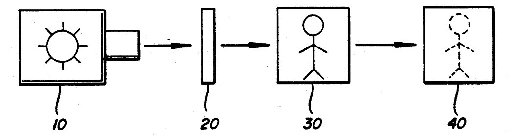
I read part of the patent and I agree that they suggest that adding this narrow filtration at approx 500 nm and 610 nm, might help reducing “problematic” regions and normalize output of different lighthouses (light sources + filtration).
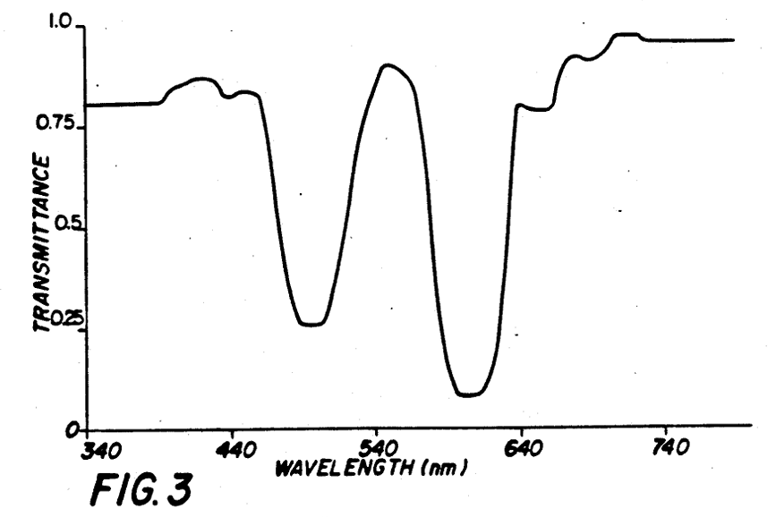
This is the recommended filter, that also will make the light source slightly warmer, reducing more of the blue part than the red.
I am curious to see also what it will do to Portra film and paper. Especially if it will make it similar to more consumer film and paper.
Thanks @NateWeatherly!
That would be amazing! Looking forward!
That’s also a great list of repositories!
Using hyperspectral images as references could be interesting and they could be used directly on the input with some hacking. Also, good databases of realistic representative spectra of real objects might be interesting to have.
Oh nice, good friends to have. I don’t have anything specific but it is good to keep in mind. Do you have any more details on their camera? I just want to geek around a bit. I guess there are many solutions to make hyperspectral images.
I guess that the physical interaction of film and print paper during the analog printing process is what we would like to preserve, because it is what encodes part of the look. It definitely encodes color shifts and style, just compare Portra and Endura Premier for example.
I am no expert, but I believe that when printing on photographic paper with modern printers and a digital workflow, the process is optimized for maximal color accuracy. In other words, printers are calibrated to match as good as physically possible the input digital RGB files and the output print colors (when the print is observed under the right conditions). Still physical limits of paper holds, e.g. white and black levels.
The challenge could be rephrased as:
In agx-emulsion, how do we make sure that the exported file, when printed on photographic paper with a modern printer, will match as closely as possible an analog print that we would make from film(+enlarger) that saw the same original scene?
With this use case in mind we should definitely put some care in deactivating part of the simulation. For example characteristic white/black levels and also glare will be already reproduced on photographic paper even with the digital printing workflow. There is nothing the printer can be about them.
For example I believe that modern printers already take into account viewing glare compensation in the best way, since they are meant to fit in a digital photographer workflow. Images are edited on screen from people that wants good results when they print.
Characteristic curves of print paper meant for analog printing for sure encodes viewing glare compensation (deeper shadows than expected because they will be brightened by glare), so we should remove it and make sure that the image we see on a calibrated screen have the shadows as deep as we would like to have.
So in summary, I think that adding black/white level controls, deactivating random glare, and using viewing glare compensation removal controls, should help in this use case. Maybe we could have an simulate_for_print checkbox that does this.
When looking at simulated images on screens we should probably emulate all paper characteristics.
Does this sound alright or am I missing something?
1 Like
i attempted an implementation of the couplers.
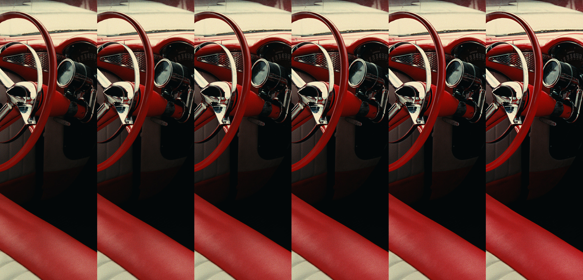
this is couplers=0.0, 0.2, ..1.0. when i look at it on my screen it increases colourfulness quite a bit… only the pixls preview looks all clamped to something. maybe my firefox tries to colour manage and fails or something. so here’s also a wedge with couplers=0.0,0.5,1.0,1.5,2.0:
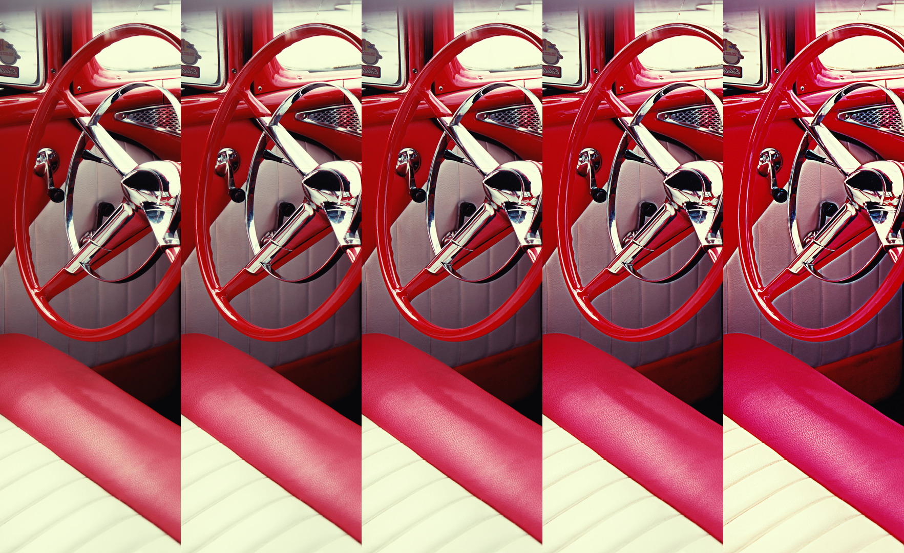
2.0 goes completely overboard, but that’s fine with me
anyhow… i’m using i think your approximations and a few on top now. one simplification is that i’m assuming the released coupler depends on the log exposure, not the density. so it’s kinda linear all the way… no saturation. not sure that breaks in some places… but it happens before the density lookup, adjusting the exposure beforehand, so it still has a soft transition to black/white.
more precisely, i’m assuming measured density curves depending on log-exposure D(e) that have been acquired using a neutral-colour test strip ramp. i’ll assume that to be locally flat/constant, or to diffuse as much into slightly darker as into slightly brighter, so the spatial diffusion kinda cancels out. In this context, the actual corrected log exposure, e_0 = e - K*e, which is reduced by a convolution of the initial exposure with kernel K in space and between layers, this reduces to only interaction with the layer diffusion matrix M, i.e. e_0 = e - M\cdot e. so what i’m claiming is that the actual density-from-exposure function D_0(e) is observed as D(e) = D_0(e - M\cdot e). this is valid only in the context of the test strip, for neutral-coloured e.
from there i compute the actual density function D_0(e) = D((I-M)^{-1}\cdot e), which will result in exactly the same result as without the couplers, but only in case e is neutral.
does that make any sense to you at all? too much approximation?
couplers M\cdot e are blurred with a radius relative to the longer side of the picture, turns out to be like 20px in normal raw images, i think. i like the local contrast increase i’m getting from large radii.
as an extra goodie, the display buffer is now mipmapped, so you can see the result of grain more realistically when zoomed out a lot. also the 2x and 4x resize works… but 4x really needs a lot of GPU memory…
didn’t push any of this yet, but will some time soon.
3 Likes
@hanatos would you have any idea what is going wrong here, trying to use vkdt filmsim, but pictures always look purple, and no amount of color or filter adjustment will fix it. Happening on two different computers too, both on OpenSUSE tumbleweed (tried AppImage and compiling) and Windows.
I have created the filmsim.lut as instructed on the GitHub page.
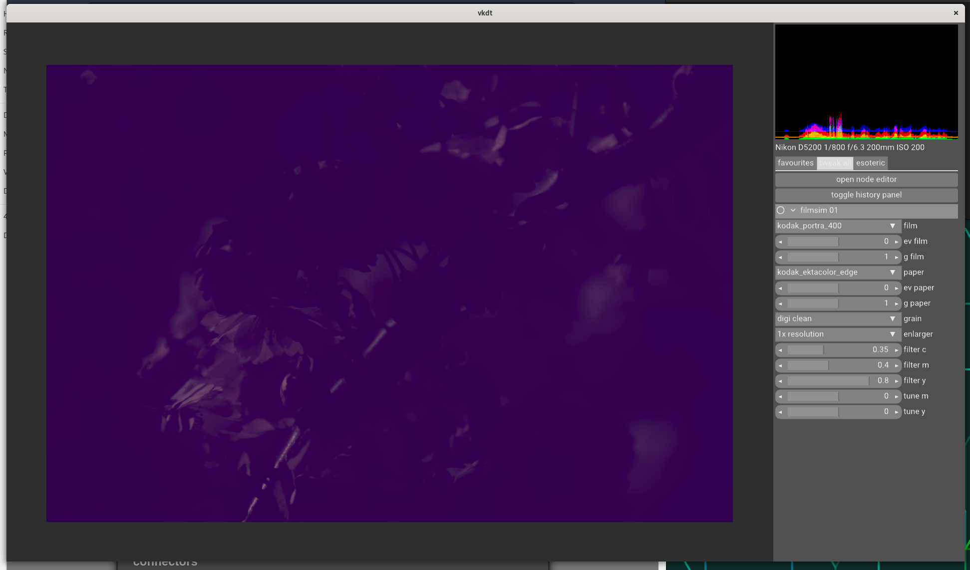
…would you have a raw + cfg file for me to see if i can reproduce?
Here you go:
_DSC0375.NEF.cfg (3.8 KB)
_DSC0375.NEF (25.5 MB)
This look actually quite promising! Considering the simplified model. 
I am a bit concerned by the whiter halos when you are pushing the inhibition, but it is probably completely overboard as you said.
I hope I got your approximations right. Here are a few comments.
I think that not saturating the amount of inhibition might violate the “conservation of mass”. I mean that in chemistry you can make as much products as the reagents can allow. If you finish reagents the reaction will stop. Since the inhibitors molecules are released when the main dyes (CMY) are produced in the emulsion, then when we reach density max it would make sense that also the inhibitors reaches a maximum. Or if no density is produced there should not be any effect of the inhibitors because they are not produced in the first place.
Using only M*e does not take into account this saturation. This might be too drastic in the region of the photos when density is saturated (before toe and past the shoulder) but still will hold fine in the linear part. So the question might be if we are fine with this approximation.
My modeling of the interlayer effects and dir couplers came also from studying some sketches from the Hunt’s book [Hunt, The reproduction of color, 6th ed, Wiley 2004]. At page 256, there is a sketch of how the interlayer effects should work on film.
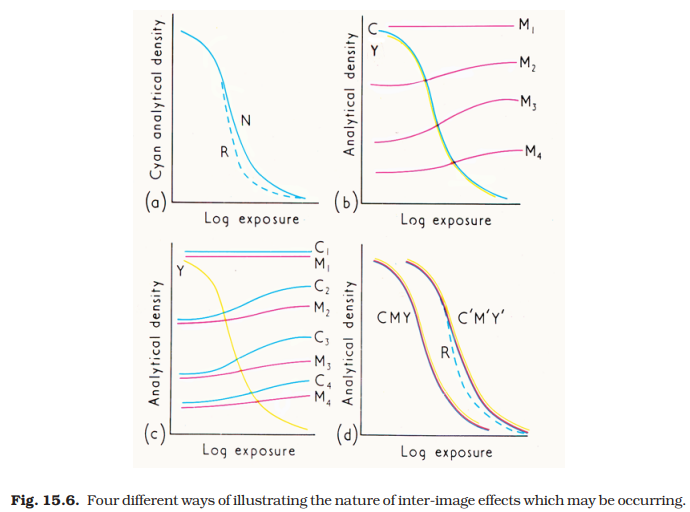
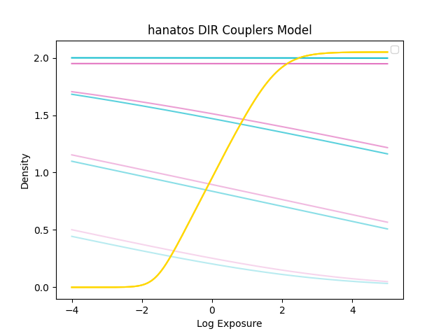
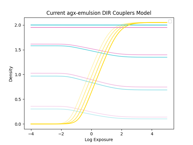
It is for positive film, but the concepts should hold. Let’s focus on panel(c), It shows a few experiments of test wedges in which the exposure of two channels (red and green, C and M layers) is kept constant while the blue exposure follows a ramp (Y layer). The final C and M density will be affected by the amount of density developed in the Y channel.
I made a small script to reproduce the experiment in panel(c) with your model and the current one in agx-emulsion.
Both models leaves unaffected density curves when a neutral ramp is used as exposure.
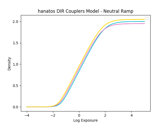
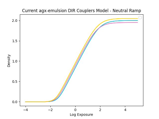
When only blue light is exposed with a ramp and the other channel with constant exposure, these are the effects.
Code for making the plots
import numpy as np
import matplotlib.pyplot as plt

def curve(e, ks):
    y = np.zeros((3, e.shape[0]))
    for i, k in enumerate(ks):
        gamma = k[0]
        e0    = k[1]
        ymax  = k[2]
        c1    = k[3]
        c2    = k[4]
        y[i] = (  gamma/c1 * np.log10(1 + 10**(c1 * (e - e0) ) )
            - gamma/c2 * np.log10(1 + 10**(c2 * (e - e0 - ymax/gamma)))
            )
    return y

k0 = [[ 0.6, -1.4, 2.00, 2, 1],
      [ 0.6, -1.5, 1.95, 2, 1],
      [ 0.6, -1.6, 2.05, 2, 1]]
k0 = np.array(k0)

N = 1024
e = np.linspace(-4,5,N) # log exposure
dc = curve(e, k0) # density curves

def plot_density(e, dc, ax=None, add_labels=True, alpha=1):
    if ax is None:
        _, ax = plt.subplots()
    # colors = ['tab:red', 'tab:green', 'tab:blue']
    colors = ['tab:cyan', 'tab:pink', 'gold']
    for i in np.arange(3):
        if add_labels==True:
            # l='RGB'[i]
            l='CMY'[i]
        else: l ='_nolegend_'
        ax.plot(e, dc[i], color=colors[i], label=l, alpha=alpha)
    ax.set_xlabel('Log Exposure')
    ax.set_ylabel('Density')
    ax.legend()

def interp_with_curves(x, e, dc):
    if np.size(e.shape) == 1:
        e = np.vstack((e,e,e))
    d = np.zeros((3, e.shape[1]))
    for i in np.arange(3):
        d[i] = np.interp(x[i], e[i], dc[i])
    return d

##############################################################################
# models

def density_dir_model_a(raw, e, dc, M):
    e = np.vstack((e,e,e)) # log exposure
    d_max = np.max(dc, axis=1)

    d_max = d_max[:,None]
    raw_mid = e - np.einsum('ck, cm->mk', dc/d_max, M)
    dc0 = interp_with_curves(e, raw_mid, dc) # density curves 0, before inhibition

    d0 = interp_with_curves(raw, e, dc)
    raw_corr = raw - np.einsum('ck, cm->mk', d0/d_max, M) # corrected log exposure

    d = interp_with_curves(raw_corr, e, dc0)
    return d

def density_dir_model_hanatos(raw, e, dc, M):
    M = M*0.1 # reduced inhibition matrix for matching roughly the models
    e = np.vstack((e,e,e)) # log exposure

    e_mid_corr = np.einsum('ck, cm->mk', e, np.linalg.inv(np.eye(3)-M))
    dc0 = interp_with_curves(e_mid_corr, e, dc) # density curves 0, before inhibition

    raw_corr = raw - np.einsum('ck, cm->mk', e, M) # corrected log exposure
    d = interp_with_curves(raw_corr, e, dc0)
    return d

##############################################################################
# test models
M = np.ones((3,3))/3

def test_models(e, dc, M, density_model, e_levels=[-1, 0, 1, 4], experiment='neutral_ramp'):
    _, ax = plt.subplots()
    alpha = [0.3,0.5,0.7,1]
    for i, ei in enumerate(e_levels):
        if experiment=='rg_constant':
            raw = np.vstack((ei*np.ones(N), ei*np.ones(N), e))
        elif experiment=='g_constant':
            raw = np.vstack((e, ei*np.ones(N), e))
        elif experiment=='neutral_ramp':
            raw = np.vstack((e, e, e))
        d = density_model(raw, e, dc, M)
        plot_density(e, d, ax=ax, add_labels=False, alpha=alpha[i])

# neutral ramp
test_models(e, dc, M, density_dir_model_hanatos, experiment='neutral_ramp')
plt.title('hanatos DIR Couplers Model - Neutral Ramp')

test_models(e, dc, M, density_dir_model_a, experiment='neutral_ramp')
plt.title('Current agx-emulsion DIR Couplers Model - Neutral Ramp')

# hunts panel(c) experiment pag 256
test_models(e, dc, M, density_dir_model_hanatos, experiment='rg_constant')
plt.title('hanatos DIR Couplers Model')

test_models(e, dc, M, density_dir_model_a, experiment='rg_constant')
plt.title('Current agx-emulsion DIR Couplers Model')
plt.show()
Tell me in case my implementation in the python code does not correspond with what you meant.
I think what is happening below log exposure = 2 (or above log exposure = 2.5) is not realistic in the sense that the Y layer cannot release inhibitors and should not affect C and M (or exhausted all the amount of inhibitors it could release on the other side). So densities of C and M dyes should not change anymore before the toe (or after the shoulder) because the Y layer is not affected anymore by the reduced (or added exposure).
Also I think that if the layers C and M can produce inhibitors they should also affect layer Y. The higher the density on C and M and the more inhibited the Y layer should be (This is not really shown in Hunt’s sketch, probably because he aligned the yellow curves to make a clearer sketch).
In my opinion, in this physically based simulations, reproducing what makes sense from a physical point of view really helps in the final look. But of course, we can take choices that helps with computational efficiency or convenience. This violate the chemical nature of the process a bit too much I think.  What’s your take?
3 Likes
hmm works for me. here’s my lut, maybe something went wrong while generating it:
filmsim.lut (144.0 KB)