Note: This post is a follow-up to The Quest for Good Color - 1. Spectral Sensitivity Functions (SSFs) and Camera Profiles, The Quest for Good Color - 2. Spectral Profiles "On The Cheap" and The Quest for Good Color - 3. How Close Can IT8 Come to SSF?" If you’re new to the series, you might want to read forward from the first post to understand what I’m doing here…
It’s amazing to me sometimes how pursuit of an endeavor can take you to places you hadn’t previously considered. It’s been a bit of time since my last post on this, but I’ve been busy trying to put a bow on the whole thing. I think the end result is satisfying, so let me describe the journey and the outcome.
In Post #2, I demonstrated a way to collect spectral data from a camera using what I’ll call the “single-shot spectrum” approach. This is in contrast to the widely accepted method of a succession of shots of single-wavelength presentations produced by a monochromator. My measure of goodness was to compare the data I collected with a monochromator-based dataset for the same camera, and it surely looked close enough. Indeed, images I developed with this new profile looked fine, and it tamed the extreme blue situation that got me started chasing this. But there were still differences, and it ate at me that there might be an affordable level of device above the coarse light box that would close those gaps. Also, it concerned me that, once I finished figuring out how close I could come for a camera for which I had reference criteria, what would I do about my Z6, for which I had no such data. Indeed, characterizing that camera is what got me going on this. So, I set out to do three things:
- Determine if simultaneous power measurement was required to produce good spectral data;
- Find out if the minimum lab-grad optical path alternative would significantly improve performance, and;
- Find a way to measure profile performance without prior reference data for the camera.
A wonderful way to wile away the COVID-19 sequester…
Power Measurement
If you look closely at the SSF comparison chart in Post #2, you’ll notice that the lower and upper curves don’t quite match the reference data. Indeed, the lower curve peaks higher, and the upper curve peaks lower. Plotting out different tungsten-halogen spectral data, there is evident a pattern of behavior, but there are slight differences. Wanting to understand if my assumption that the Open Films Tools DedoLight data sufficiently characterized tungsten-halogen light, I set out to find a way to measure my LowellPro light. Keeping true to my minimal-cost mantra, my first excursion was to build a spectrometer. This turns out to be a rather popular thing to do, with dozens of recipes for such all over the internet. The best source of information I found was at https://publiclab.org/, where they took the concept well-past the cardboard-and-dvd-diffractor stage of the rest (indeed, I found information there significant in other ways, as you’ll later see…).
Such a device is based on a camera; indeed, commercial spectrometers have a one-pixel-high array much like a camera sensor upon which a diffracted beam is splayed. I decided to restrict my search to Raspberry Pi cameras, as I have a few of those boards laying about and I speculated that hosting some of the procesing there would be effective. Indeed, before I was done with the excursion, I had built a web-based spectrometer application. Geesh…
Thing is, a device that measures power has to have the same sensitivity across the visible spectrum. What vexes this need is the CFA filtration in most cameras. So, I spent time looking for small, inexpensive monochrome cameras. Before that, I considered scraping the CFA array off of the Pi camera I already had, but abandoned that thought after reading the exploits of others who borked up to 7 cameras before they got one that still worked after the surgery. Anyway, fortune came my way in the form of a RPi-compatible monochrome camera from ArduCam. This one: Arducam OV7251 0.31MP Monochrome Global Shutter Camera Module for Raspberry Pi 4/3B+/3 - Arducam . It’s only a 640x480 pixel camera, but I figured I didn’t need much resolution to measure what’s effectively a right-to-left mostly linear downslope through the visible spectrum. Using patterns observed at publiclab.org, I put together a spectrometer using small poplar stock from the local home store. With it and my horrid-hacked spectrometer webpage I was able to capture spectra like this:

This is spectra from the CFL bulb I use for calibration. Note that it’s not colored, that’s in keeping with the un-colored-ness of light, and the corresponding single-channel data from the mono camera. Pertinent to my objective, not having a CFA meant the measurements at each wavelength were taken at the same sensitivity, and so the plot represents relative energy at each wavelength. Don’t have to measure a quantity such as lumens, just need to get a normalized dataset of relative values for compensating the SSF measurements.
Here’s my first tungsten-halogen power measurement:

Well and good, except for one thing: it truncates at 650nm. Tungsten-halogen spectrum has power well into the infrared, but this device won’t measure it. The camera has a 650nm IR filter, dang. I tried to pry off the lens cover to remove it but that thing is fastened too well to even get a knife blade in the crack. I also considered extrapolating the peak to 730nm, the minimum upper end of the visible spectrum, but that’s where the data rolls off to the descent into infrared and any attempt I made to approximate it did not end well in the resulting SSFs. All of this was pointing to procuring a spectrometer, but I wasn’t ready to do that yet so I put this excursion aside…
Lab-Grade Optical Components
I just couldn’t shake my trepidation regarding a diffraction grating consisting of a cheap piece of plastic with printed grooves mounted in a cardboard slide mount. Even though I could easily see that my measurements were pretty close, I wanted to take the next step to see what kind of difference it would make. So, I broke out the credit card and ordered a diffraction grating and diffuser from Edmund Optics. Here’s what I procured:
Note the prices. Edmund sells a 12.5mm grating for about $85US, but that just seemed too small and the 25mm grating was only about $30US more. The size OpenFilmTools used, 50mm, is over $200US, so I made a judgement call picking the 25mm one as the best trade between price and potential. The 25mm diffuser was only about $15US; for reasons I’ll explain later, at that price I’d just get one of these even to use with the cheap diffraction grating.
I looked at the lab-grade optical slits, but > $100US just seemed such a stretch for something with which I wanted to play with the width, so I settled on a fabrication that held two razor blades to make the desired aperture.
The size of the grating concerned me, as it was a quarter the size of the cardboard-plastic grating and I didn’t know the geometric considerations of the size difference. Indeed, I could not find any literature on that. Turns out it does seem to make a difference on how far the lens focal length can be before the ends of the spectrum start to fall off. Anyone who knows how that works, please feel free to pipe up…
In considering things about using a diffraction grating, I found the information at publiclab.org to be quite instructive, particularly this post:
Of particular importance, the grating spacing does have a defined relation to the spectrum spread. That relation is described in The Grating Equation, here’s the form of the equation that solves for the diffraction angle:
where:
d = grating groove spacing
a = diffraction exit angle
i = angle of the incoming light (incidence angle)
w = wavelength of light in nanometers
I found this form of the equation so useful I coded it in C++ and used it to do some analysis:
float angle(float w, float d, float i, float o=1.0)
{
	w /= 1000000; //whole unit to fraction
	return (180/pi)*(asin((o*L*d)-(sin(i*pi/180))));
}
o is the diffraction order, if one needs that; most of what we’re considering is in the first order. Note the fraction conversion, the caller specifies the wavelength in whole numbers of nanometers, but the value to the calculation has to be a proper fraction of a meter. Also note the degree->radian and radian->degree conversions to accommodate the math library calls;
stoft, the writer of the publiclab post, observed that the original publiclab spectrometer design produced a skewed spectrum, which affected the alignment to the linear wavelength calibration. After looking at that for a while, it occurred to me that the spectroscope design I implemented in my first box had the same affliction, given its incidence angle of zero. stoft proposed a 45-degree incidence angle for their spectrometer redesign; I chose to work through the numbers to find the appropriate angle to put the center of 380-730nm equidistant from those two bounds. A bit of spreadsheeting of iterations of angle() determined the closest whole-number angle to do this was 42 degrees. The whole-number is significant in that I’m using a carpenter’s chop saw to cut the relevant angle, and I didn’t want to do eyeball interpolation between its angle marks. Here’s a GIF animation of the relation of the incidence angle to the spectrum spread about the mid-point:

So, instead of mounting the grating to take the light head-on, I moved it to the angled wall and now the camera looks directly at the grating face and straight-on to the spectrum midpoint. This will make assigning wavelength values to the columns of the spectrum more accurate.
I picked 1200 grooves/mm for my procured grating because it would produce the largest spread of the spectrum across the pixels.
Now, my immediate objective was to compare performance of lab-grade and school-grade optical components, which implied an equivalent design change for the plastic diffraction grating. So, I did the angle analysis for the plastic grating’s 1000 grooves/mm, and came up with the angle 34 degrees. With this information I built two boxes, with the respective angles for their diffraction gratings. This also allowed me to design fixtures for the slit and diffuser that would fit either box, so I could mix and match to determine their respective contributions in either configuration. Well, ended up building a few other aborted boxes, one which had the angle (42 degrees) oriented wrongly for mounting on my desk. Good thing poplar is relatively inexpensive…

Here are the two boxes, looking into the camera ports. Note the difference in angle, as discussed above. The optical-grade grating is on the left. Also note the extension of the camera face below the table surface; this helps to orient the box on the table and keep it oriented. I considered drilling holes to bolt it to the table, but it turns out it’s rather handy to center the spectrum on the sensor by sliding the box from side to side, registered in the other orientations by that flange.
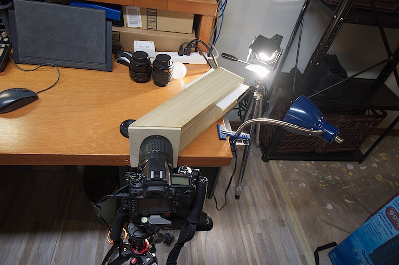
Here’s the entire optical chain in action. This is the 42-degree box, with the optical-grade grating. The overall setup is pretty much the same as was in Post #2, with the LowellPro tungsten-halogen spot and the CFL calibration bulb in the blue goose neck fixture.
There’s a whole calculus of slit width/length, slit-grating spacing, camera-grating distance, and lens focal length of which I only have a notional understanding at the time of this writing. I may make yet other boxes, depending on what is concluded in the next section…
Measuring Performance
dcamprof and dE
The comparison plots of the spectrum-measured data with the monochromator-measured data for the Nikon D7000 are insightful, but of really no use moving on to other cameras. Realizing this, I figured it was time to dig into the data produced by the dcamprof -r command line parameter. When ‘dcamprof make-profile -r reports …’ is run, dcamprof creates the reports directory and dumps a whole bunch of data and pictures depicting various characteristics of the created profile. Since the previous command, ‘dcamprof make-target … -p cc24’ uses the ColorChecker 24-patch reference spectra to produce the synthetic target, dcamprof produces a number of patch-errors files, depicting various differences between the patch colors rendered by the created profile with their reference values. The value reported in these files is ‘delta-E’, or dE, or DE, which is defined as the discernible difference between two colors, with the value 1 representing the minimum human-discernible difference. The file ‘patch-errors-txt’ contains these values for each of the 24 patches. With this, we have a way to evaluate each created profile against spectrometer-measured reference values for a color target.
Of even more use is a related file, ‘patch-errors.tif’. This TIFF image contains the DE values for each patch, as well as a square patch diagonally divided into two parts: 1) the color of the reference value, and 2) that same color rendered through the profile. Allows one experience DE, directly. The TIFF is rendered in linear ProPhoto, so it needs to be viewed with a color-managed viewer. Here, I converted one to sRGB in the hope the differences are appropriately apparent:

This report is from the monochromator rawtoaces profile. With this, we now have a camera-independent objective, max DE of 2.76, in this case for the C04 patch. For perspective, maximum DE for my D7000 matrix profile from a ColorChecker Passport shot is 5.95.
The “Cheap” vs “Cadillac” Shootout

On the left, a 25mm square of etched glass, $108US. On the right, a piece of plastic with printed lines mounted in a cardboard slide holder, package of 5 for $3US.
And now we come to the whole reason for this missive - determining if spending a bunch of money on lab-grade components is worth the difference in performance. Before we get to that, a few words about tools. In Post #2, I described ssftool, a command-line program I wrote to process spectral data extracted from an image into SSF data digestible by dcamprof. Since that post, I’ve put a lot of work into ssftool, particularly with the wavelengthcalibrate operator. It does a linear interpolation between the pixels with the known wavelengths, so it’s imperative that the spectrum splays linearly on the camera sensor. I reworked that routine to be more accurate per-wavelength, which complements the symmetric distribution of the spectrum achieved with the 42-degree incidence angle. I also wrote a special version of the crop tool for rawproc, specifically for the img command line processor, called ‘cropspectrum’. This tool extracts a spectrum from an otherwise dark image by finding the max green pixel, then extracting the row band based on the center of the surrounding column. With img, ssftool, and dcamprof I wrote a script to process from the raw spectrum and calibration files to a profile and it’s associated reports in about 10 seconds on my 4-core Phenom machine. Those interested in the algorithm can regard it here: rawproc/gimage.cpp at master · butcherg/rawproc · GitHub
By the way, ‘cadillac’ is an American euphemism meaning ‘top-grade’. Back in the day, any motor car carrying the Cadillac name was considered by the public at large to be the pinnacle of automotive ownership. My dad aspired to own a Cadillac; by the time he could afford such, the brand was in decline. In describing this approach with lab-grade opticsvI was looking for a euphemism for ‘fancy’, and ‘cadillac-components’ just seemed right…
For image capture, I’ve used a tethering program. I started with QDSLRDashboard in Post #2, but for #4 I wanted to capture the raws directly to my linux box and I wanted something simpler. That software proved to be Entangle, which installed from the Ubuntu repository. It’s not much use for focusing as the JPEG-quality live view usually blew out most of the spectrum, but being able to directly capture NEFs to a directory for processing saved a bunch of time. It does crash a bit, one time rebooting my machine, but not so much that it adversely affected my ability to rapidly turn profiles. The only good way to focus is through the viewfinder, or in a good LiveView on the camera back.
Good thing I had such a tool chain, because I proceeded to take somewhere in the neighborhood of 50 spectra over the course of a couple of days, trying various combinations of lens focal length, exposures, and optical components to find the best performance. Interestingly, the very first ‘cheap’ profile I created was the best of that class, max DE 2.93. Here’s the full sorted-by-DE report:
  D02 DE 0.00 DE LCh +0.00 +0.00 +0.00 (gray 80%)
  D03 DE 0.13 DE LCh -0.01 -0.12 -0.05 (gray 70%)
  D04 DE 0.14 DE LCh -0.01 -0.04 -0.14 (gray 50%)
  D06 DE 0.15 DE LCh +0.02 -0.15 +0.02 (gray 20%)
  D05 DE 0.20 DE LCh -0.00 -0.09 -0.18 (gray 40%)
  A01 DE 0.59 DE LCh -0.00 +0.30 +0.51 (dark brown)
  D01 DE 0.71 DE LCh -0.11 -0.67 -0.23 (white)
  A06 DE 0.86 DE LCh +0.03 -0.23 +0.83 (light cyan)
  A04 DE 1.08 DE LCh -0.82 +0.69 -0.04 (yellow-green)
  A03 DE 1.13 DE LCh +0.90 -0.60 -0.57 (purple-blue)
  A02 DE 1.27 DE LCh +0.58 -0.02 -1.13 (red)
  B04 DE 1.43 DE LCh +0.87 -1.13 -0.14 (dark purple)
  A05 DE 1.51 DE LCh +1.14 -1.08 -0.25 (purple-blue)
  B03 DE 1.55 DE LCh +1.46 -0.28 -0.43 (red)
  B01 DE 1.75 DE LCh -0.23 -0.56 -1.64 (strong orange)
  B02 DE 1.80 DE LCh +1.71 -0.89 -0.91 (purple-blue)
  B06 DE 1.81 DE LCh -0.84 -1.42 -0.75 (light strong orange)
  C02 DE 2.02 DE LCh -0.64 -1.57 +1.11 (yellow-green)
  C01 DE 2.11 DE LCh +1.97 -1.00 -1.14 (dark purple-blue)
  C03 DE 2.31 DE LCh +1.92 -0.83 -0.99 (strong red)
  C06 DE 2.48 DE LCh +1.93 -0.71 +1.38 (blue)
  C05 DE 2.85 DE LCh +2.22 -1.31 +1.21 (purple-red)
  B05 DE 2.88 DE LCh -1.38 -2.34 +0.96 (light strong yellow-green)
  C04 DE 2.93 DE LCh -0.88 -2.76 -0.44 (light vivid yellow)
I struggled with the ‘cadillac’ collection; it took a bit to figure out which focal lengths didn’t truncate the ends of the spectrum, probably a good reason to consider a larger grating. 18mm, the widest focal length on the 18-140mm lens, produced the best max DE at 2.80. Here’s the full sorted-by-DE report:
  D02 DE 0.00 DE LCh +0.00 +0.00 +0.00 (gray 80%)
  D03 DE 0.12 DE LCh -0.01 -0.11 -0.03 (gray 70%)
  D04 DE 0.13 DE LCh -0.02 -0.04 -0.12 (gray 50%)
  D06 DE 0.16 DE LCh +0.01 -0.16 +0.00 (gray 20%)
  D05 DE 0.18 DE LCh -0.01 -0.09 -0.16 (gray 40%)
  A01 DE 0.35 DE LCh -0.08 +0.22 +0.27 (dark brown)
  D01 DE 0.70 DE LCh -0.11 -0.66 -0.19 (white)
  A06 DE 0.87 DE LCh +0.18 -0.18 +0.83 (light cyan)
  A02 DE 1.14 DE LCh +0.58 -0.20 -0.96 (red)
  A04 DE 1.15 DE LCh -0.85 +0.77 -0.02 (yellow-green)
  A03 DE 1.16 DE LCh +0.99 -0.46 -0.60 (purple-blue)
  B04 DE 1.37 DE LCh +0.74 -1.14 -0.26 (dark purple)
  B03 DE 1.39 DE LCh +1.31 -0.43 -0.14 (red)
  A05 DE 1.53 DE LCh +1.17 -1.10 -0.32 (purple-blue)
  C02 DE 1.64 DE LCh -0.51 -1.24 +0.95 (yellow-green)
  B01 DE 1.82 DE LCh -0.47 -0.43 -1.71 (strong orange)
  C03 DE 1.83 DE LCh +1.68 -0.65 -0.34 (strong red)
  B02 DE 1.88 DE LCh +1.78 -1.06 -0.75 (purple-blue)
  B06 DE 1.88 DE LCh -1.09 -1.23 -0.91 (light strong orange)
  C01 DE 2.12 DE LCh +2.05 -0.82 -0.52 (dark purple-blue)
  B05 DE 2.69 DE LCh -1.42 -2.09 +0.92 (light strong yellow-green)
  C05 DE 2.75 DE LCh +2.04 -1.47 +1.13 (purple-red)
  C06 DE 2.75 DE LCh +2.29 -0.95 +1.15 (blue)
  C04 DE 2.80 DE LCh -1.03 -2.57 -0.43 (light vivid yellow)
I did try various combinations of better slit and diffuser with the cheap grating, and the most noticeable benefit came from the diffuser. It let more light through to the slit than the paper, which made focusing easier. The slit proved more challenging to evaluate, mostly because my cardboard razor blade holder didn’t hold the blades too tightly. I saw a neat slit design that used those new powerful magnets, on my to-do list.
After a lot of messing around with camera alignment, I found the best way to do it was to 1) level the tripod head, my head has one of those circular bubble levels that help that; 2) for a zoom lens set the lens focal length, do this now because that likely affects the physical lens length; 3) set the elevation so the lens center is level to the grating center; 4) slide the camera up to the box face, centered on the opening; 4) viewing the spectrum in the tether program, tilt the camera until the spectrum is level; 5) turn off the tether, then looking in the viewfinder or liveview, slide the box left or right on the table edge until the edges of the spectrum are both in the frame, you’ll see them fade off as you move too far left or right; 6) focus using the viewfinder/liveview.
Choosing a focal length will probably take some experimentation; start with smallest, then work up until you find the sweet spot between coverage and falloff.
Conclusions
Well, the big and somewhat surprising conclusion is that the cheap grating provides acceptable results. With a decent diffuser, that keeps the whole contraption under $30US. The box isn’t that difficult to fabricate; I tried to keep the cuts simple to limit the requirednpower tools to a radial chop saw and a drill with a couple of hole saws.
Of note is that the better grating really does not significantly improve the performance. Indeed, the DE difference between the monochromator reference and either whole-spectrum box isn’t that great.
The big challenge is alignment, but I found that becomes easier as one sees the dynamics through the viewfinder. After shooting targets, I think those challenges are more manageable than controlling glare.
The above-described profiles were power-adjusted with the same DedoLight data used in Post #2. Given the profiles’ DE performance, my take on power calibration is that, at least for tungsten-halogen illumination, a generic dataset is good to get one “close enough”. This is important IMHO, as the added cost to measure power while collecting spectrum would far outstrips the cost of the lightbox. Also regarding calibration, I considered other influences such as the diffuser and the camera lens, but I think their non-linear influence is not significant enough to address.
Perspective
If the camera manufacturers provided this data with their cameras, we wouldn’t have to consider doing stuff like this. But most don’t so here we are - looking for the price-point of a viable means to measure the few cameras we each own. But you know, there’s a lot to be learned doing this sort of work, not the least finish carpentry  For me, it was during this campaign I came to really understand the difference between light and color. And, I now have decent LUT camera profiles for all my cameras.
I have some residual work to do on this, particularly making a .pdf how-to on lightbox construction and writing a tiff2specdata program to extract data from an image without having to take on rawproc. Both will become a part of the ssftool github repository, at GitHub - butcherg/ssftool: command line tool to transform spectral measurements into data for use in creating camera profiles.. But, I think this post is the end of this particular series; thanks for reading!
