While looking for a decent in-camera ASIC processed monochrome solution for quickly posting images while I’m away from the Big Computer, I fell down a rabbit hole labeled Zone System. I realize it’s a well trodden path, but I found a few things that surprised me.
Setting Zone 5 to EV0 seemed a natural enough reference point. But in doing that the highlight region is attenuated by 1EV/1f-stop where Zone 9 becomes pure white instead of Zone 10 as originally described by Adams/White/Picker. This simple observation helps explain to me why the vast majority of digital black and white shows an unfortunate lack of highlight separation.
On the other hand, digital shadow tones seem to “go on forever” where usable image information is often found down in Zone -2 (which isn’t described in the original system) and slightly beyond.
So, to balance digital highlights and shadows I tried setting -1EV to Zone 5 (127decimal/7Fhexidecimal) and fit an input correction curve from Zone -2 through Zone 8 at precise 1EV intervals. This seems to solve a whole range of issues I’d experienced processing digital black and white.
Using RawTherapee I am able to insert an input correction curve just after demosaicing and just before any Camera Profiles are applied. In fact, I turn off Camera Profile “Tone Curves” and rely on the correction curve I calculated during the Zone realignment process.
I realize this probably sounds like a whole bunch of Hoo-Haa, but it works for me. I can finally get digital to look/behave like film did back in the day when dinosaurs roamed the earth.
Anyways, I wrote about this on my blog. There are a few details that I wanted to record for future reference (I’m getting old and easily forget things). The entire journey is currently linked on the upper right side of the blog page.
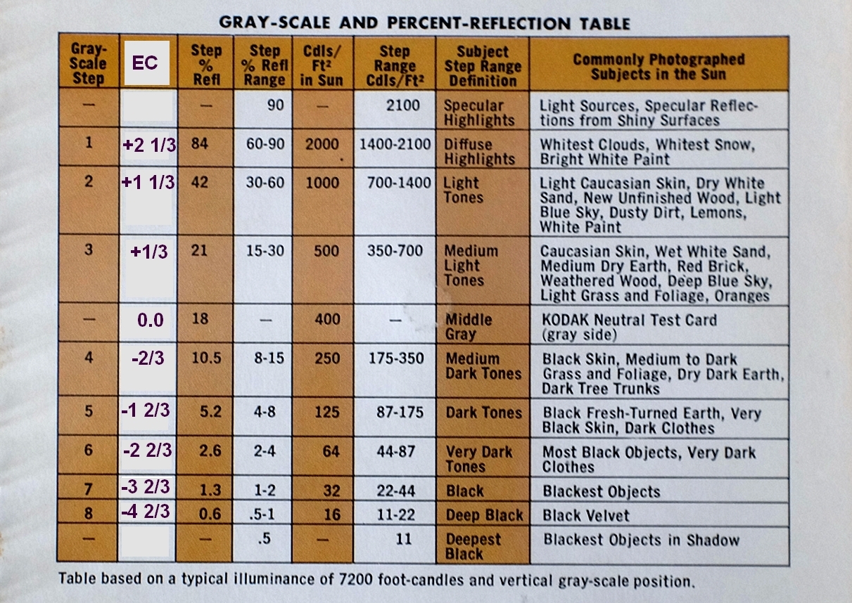
I edited an unwanted column to show exposure correction relative to mid-gray. Of interest is the relationship of the first up/down steps from middle gray which are not the same as Adams’ + and - 1 EV (see EC column).
As to outdoor scenes with cloudy skies, I am rather fond of a reverse ‘S’ tone-curve which increases cloud-contrast and brings out shadows a bit.
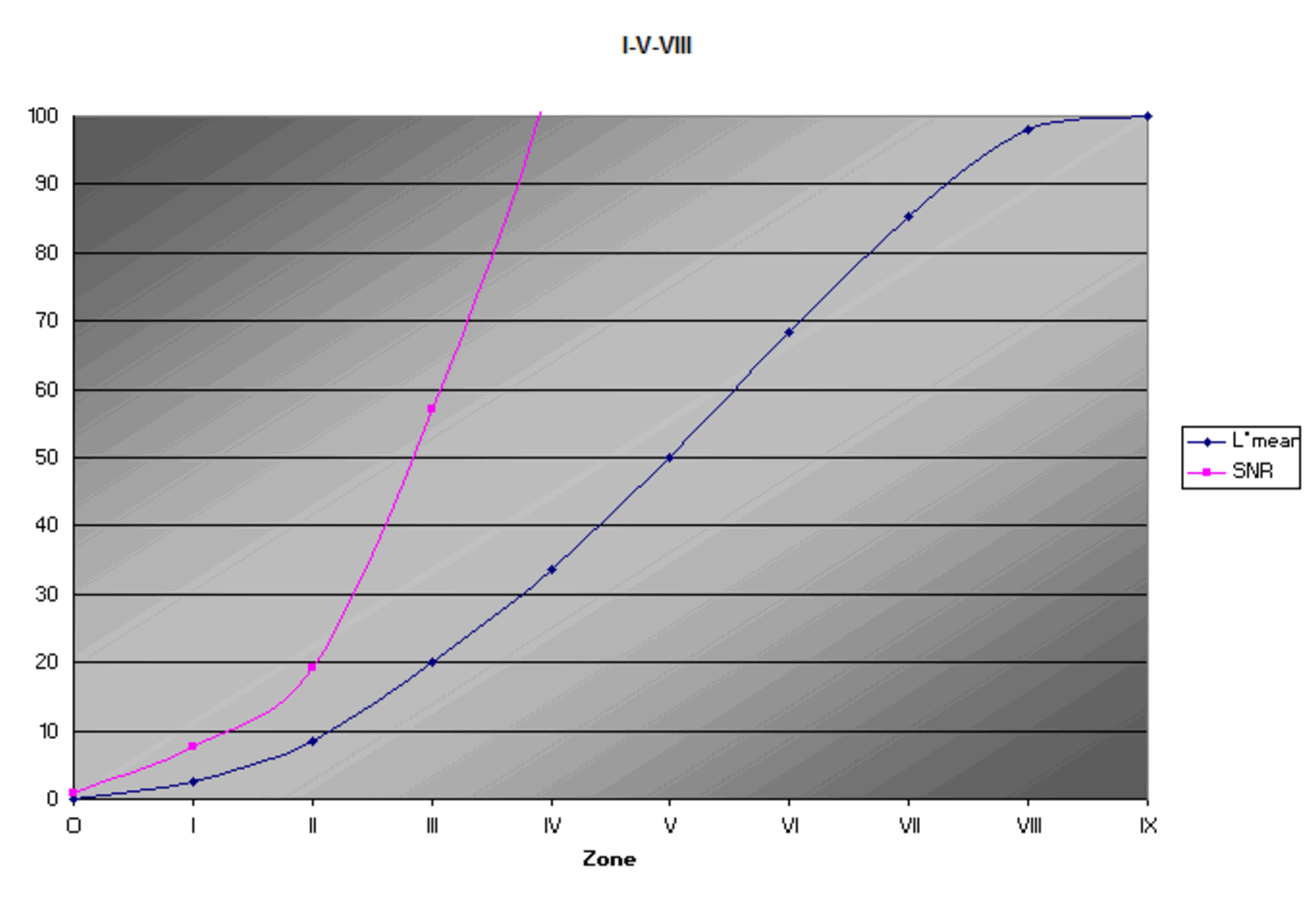
Back to Zones, here’s a Sigma/Foveon camera response curve (mean Lightness v. Zones).
@anon8280290 - This is very very interesting. I wonder what the reasoning was for the less than 1EV step between Zones 4 and 5, and then Zones 5 and 6???
Coming from film I find I prefer a bit more tonal separation in the highlights, since, as you already know, film had a really gentle and long shoulder into the pure white.
However, I’m also interested in understanding the details of the interpretation you shared here, since this seems to be what current digital work is based on, instead of Zone 10 being pure white.
I think it’s probably worth mentioning that Zone IX was defined as pure white until Adams’s last round of revisions, c. 1980, when Zone X was promoted to the Normal scale. There are also curiosities in some of Adams’s illustrations that might suggest his definition of white may have been lower than Zone IX at some point.
The copy of the table I have is in the Kodak Professional Photoguide. It is intended to be used with an accompanying set of grayscale steps that are printed on photo paper, and used for setting up a standard processing workflow. Instead of being referenced to middle gray, they “hang” from reference white (100% diffuse reflectance). The lightest step has a density of 0.03 (0.1 EV) below paper white, analogous to Zone VIII if Zone IX is white. (Note that the non-zero values given in the EC column appear to off by about 0.11 EV.)
I found the table and gray steps to be unnecessarily confusing, and used the Q-13 gray scale instead.
Taking “middle gray”/7Fhex/127dec as a starting point, in both the Gimp and RawTherapee I increased/decreased by adjacent 1EV exposure values. I did this to try and understand what the software is doing. This became my digital reference as it gives me the 1EV separation values that I apply to an input correction curve. Here’s what I see - https://flic.kr/p/2qdUCj3 It looks remarkably similar to the Sigma curve.
I never knew this. It’s likely due to where I started - Minor White’s “Zone System Manual.” I’ll have to think about this a bit.
To confirm for myself the potential value of setting a digital input correction curve to -1EV as Zone 5 and Zone 10 as pure white, I took a look at highlights. Here’s what I found - https://flic.kr/p/2qkTvaj For me, understand higher contrast situations, this looks like a useful gain in highlight tonal separation.
“middle gray” is generally accepted as being 18% reflective. With camera sensors having about a linear response, middle gray should give a raw value of 0.18 where 1 = fully exposed. When converting raw to 8-bit sRGB, it is necessary to apply gamma, approx 2.2, so 0.18^(1/2.2) = 0.461 x 255 = 117.55 or 118 rounded up.
Going the other way from your middle gray, 127/255 = 0.498^2.2 = 22% - well over the generally accepted 18%.
I see the difference between our numbers. I used 0EV metered in-camera to define “middle gray.” The answer always comes out 7Fhex for me. I guess I’ll have to think on this one a bit longer.
I’ve not found this to be exactly the case. Software automation messages images more than I expected. Looking at post demosaic/pre-Camera Profile image shows non-linearity. It’s more like a concave curve at that point. How much non-linearity depends on the generation of the sensor from what I’ve seen so far.
Your camera metering matches the type of ISO exposure index used by the camera manufacture. I am quoting the type called SOS (standard output sensitivity). An earlier type gives some headroom in the shot causing an output of about 90/255. The most common type these days is REI (recommended exposure index) for which there is no standard output for middle gray, it’s whatever the manufacturer or Chuck Norris thinks is best for you. On top of that, ISO allows a latitude of about +/- 10%, so the output can vary from camera model-to-model.
In other words, although ‘Metering 101’ says that it tries to set any scene to middle gray, the result is quite variable in practice.
Since we are talking about “raw” data written to the card, the difference is more likely due to pre-processing applied to the sensor outputs than it is to different sensor technologies, IMHO.
Thank you for making this point. It got me to reading and studying a little more deeply.
Upon closer inspection I found an error in my thinking and processes. I’ve improved my understanding and have applied the needed modifications to my input correction curves.