Hi, trying around with function edgels (aim to work a bit with curvature), I see frequent neighbored edgels with equal coordinates and different normal. Is that intended? No simple deviation possible!
Hello Karsten,
Yes, an edgel is defined by the (x,y) coordinates of its associated pixel, as well as the direction number (0,1,2 or 3), that defines which edge of the pixel the edgel represents (North, East, South or West).
When you are following a contour path with edgels, it’s then definitely common to have a sequence of edgels that share the same pixel but with different orientations.
Imagine for instance a pixel located at the end of a line, the edgels will turn around this pixel when you follow its contour.
Thank you, David, for the explanation.
Definitely the sequence of edgel pixel coordinates is not sufficient to identify the contour, e.g. for fourier shape analysis. I think I have to meditate about pixel corner locations (and edgels of voids).
I am interested in what you are working on @KaRo with edgels.
Why that ? A sequence of edgels usually starts from one point and go back to it, so it’s a very good way of parameterizing your contour, with (t,x(t),y(t)), and it even has a kind of “sub-pixel” precision, as for one pixel you have 4 possible sub-steps.
If you take an edgel sequence, keep only the x(t),y(t) components of each edgels, and “discard” the possible repetitions of these x,y, you’ll get an accurate sequence of contour points.
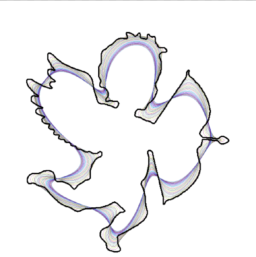
Here is a simple example of a command that parameterize a contour curve, by extracting the pixel coordinates using edgels.
Once you have the curve parameterization, you can do whatever you want (here I’m displaying smoothed versions of the curve, but you can of course do curve analysis).
foo :
  shape_cupid 512

  # Find random starting edgel (not optimal!).
  x,y,n:="do (P = int(u([w,h])%[w,h]), !i(P) || (V = crop(P[0]-1,P[1]-1,3,3);V[1] && V[3] && V[5] && V[7]));
          [ P, !V[5]?0:!V[7]?1:!V[3]?2:3 ]"

  1,1,1,2 # Will store the sequence of edgels
  eval ${-math_lib}" # Loop over all contour pixels (discard edgels with same (x,y) coordinates).
    P0 = P = [ $x,$y,$n ]; # P0 = Starting edgel
    prev_xy = [ -1,-1 ];
    do (xy = P[0,2]; prev_xy!=xy?da_push(xy); prev_xy = xy; P = next_edgel4_fg(#0,P,1); _(while) P!=P0); da_freeze()"

  # Smooth now parameterized curve at different levels and display corresponding contours.
  {0,2*[w,h]},1,3,255
  [1]
  repeat 30 {
    eval. "begin(col = [u,u,u]*255); P = 2*I; pP = 2*J[-1]; y>0?polygon(#-2,2,pP[0],pP[1],P[0],P[1],0.5,col); I"
    b. 0.5%,2
  }
  rm.

  eval[1] "P = 2*I; ellipse(#-1,P[0],P[1],2,2,0,1,0)" # Larger outline for original contour
  r2dx. 50%
And the corresponding video:
Thank you again, David!
Your shown example is a bit above my gmic math. processor usage level.
However, interesting and helpful, also for my learning curve.
It shows really nicely the curve smoothing. For shape differentiation (describing/quantizing) possibly area or the contour length should be constant. But that gives not such visually nice “potential” lines.
Concerning the curve filtering (here blurring) I have to think about the sample points not aequidistant on the contour (distance 1 or sqrt(2)).
Actually I am playing again around with phytoplankton recognition, a quite old data set.