Always good to go off in orthogonal directions, if for no other reason than to see where you’ve been from a new perspective.
So — in that spirit — lets revisit Ribbons:
splinefun.gmic
===
ribbons:
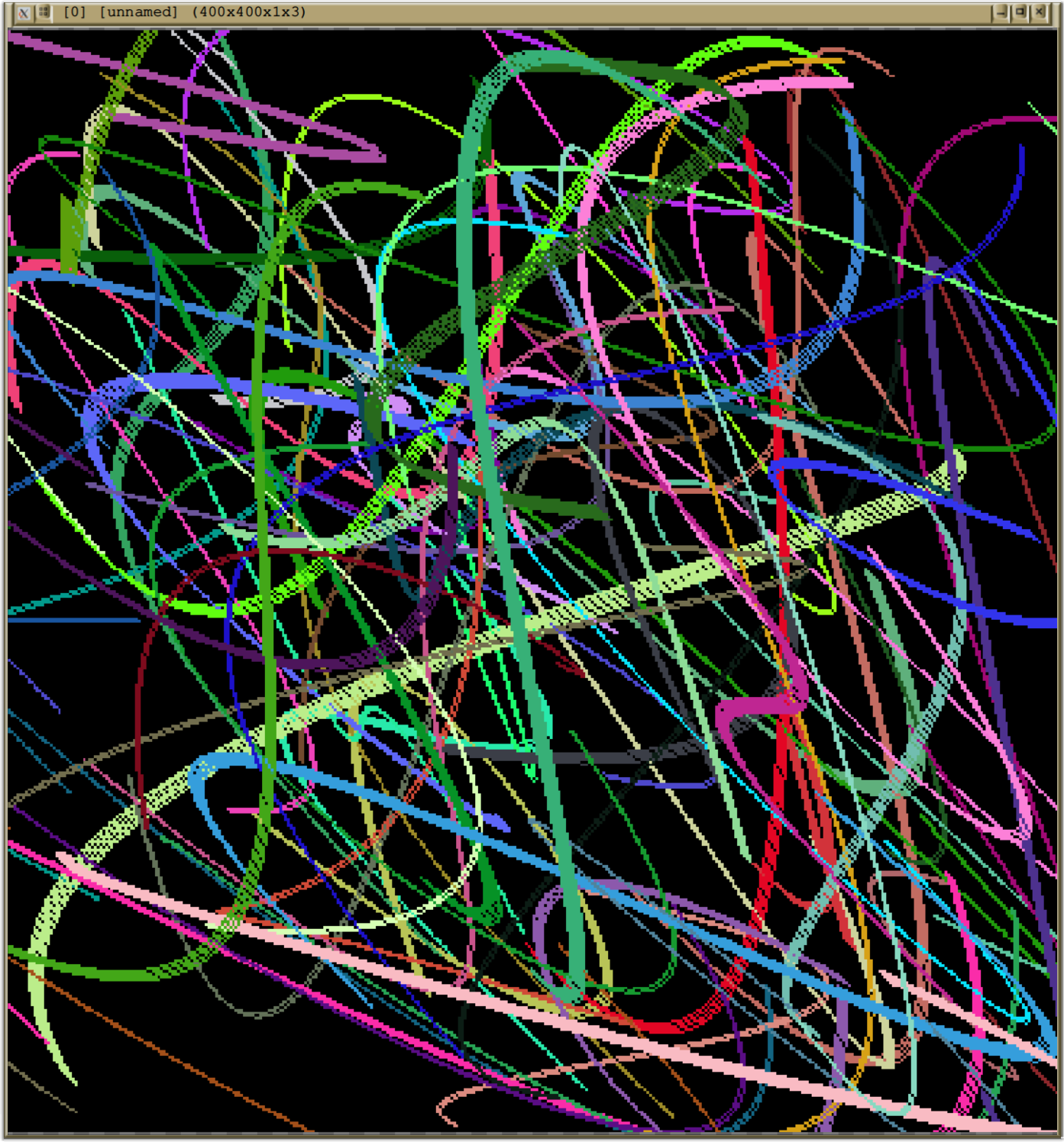
# Mediumres, 235 curves, 50% opacity and complex...
ccnt=235
-input 1024,1024,1,3,lerp([20,17,38],[33,38,46],y/(h-1))
-name canvas
(252,233,59^115,22,210^22,210,186)
-permute. cyzx
-resize. $ccnt,1,1,3,3
-name palette
-splinefun[canvas] [palette],128,5,3,65,0.5
-keep[canvas]
-text_outline. "Mediumres,\ 37 curves,\ 50% opacity\ and\ complex...",3%,90%,3%,1,1,255,240,200
-text_outline. "Spline\ Fun:\ 128,5,3,65,0.5",3%,95%,3%,1,1,255,240,200
-output[canvas] /dev/shm/ribbons_00.png
-rm
# Mediumres, 37 curves, opaque and simple...
ccnt=37
-input 1024,1024,1,3,lerp([20,17,38],[33,38,46],y/(h-1))
-name canvas
(252,233,59^115,22,210^22,210,186)
-permute. cyzx
-resize. $ccnt,1,1,3,3
-name palette
-splinefun[canvas] [palette],64,3,9,65,1
-keep[canvas]
-text_outline. "Mediumres,\ 37 curves,\ opaque\ and\ simple...",3%,90%,3%,1,1,255,240,200
-text_outline. "Spline\ Fun:\ 64,3,9,65,1",3%,95%,3%,1,1,255,240,200
-output[canvas] /dev/shm/ribbons_01.png
-rm
# Coarse, 8 curves, 25% opacity and simple...
ccnt=8
-input 1024,1024,1,3,lerp([20,17,38],[33,38,46],y/(h-1))
-name canvas
(252,233,59^115,22,210^22,210,186)
-permute. cyzx
-resize. $ccnt,1,1,3,3
-name palette
-splinefun[canvas] [palette],16,2,24,15,0.25
-keep[canvas]
-text_outline. "Coarse,\ 8 curves,\ opaque\ and\ simple...",3%,90%,3%,1,1,255,240,200
-text_outline. "Spline\ Fun:\ 16,2,24,15,0.25",3%,95%,3%,1,1,255,240,200
-output[canvas] /dev/shm/ribbons_02.png
-rm
# Hires, 256 curves, translucent and simple...
ccnt=256
-input 1024,1024,1,3,lerp([20,17,38],[33,38,46],y/(h-1))
-name canvas
(252,233,59^115,22,210^22,210,186)
-permute. cyzx
-resize. $ccnt,1,1,3,3
-name palette
-splinefun[canvas] [palette],256,3,3,45,0.125
-keep[canvas]
-text_outline. "Hires,\ 256\ curves,\ translucent\ and\ simple...",3%,90%,3%,1,1,255,240,200
-text_outline. "Spline\ Fun:\ 256,3,3,45,0.125",3%,95%,3%,1,1,255,240,200
-output[canvas] /dev/shm/ribbons_03.png
-rm
# Very hires, 512 curves, very translucent and complex...
ccnt=512
-input 1024,1024,1,3,lerp([20,17,38],[33,38,46],y/(h-1))
-name canvas
(252,233,59^115,22,210^22,210,186)
-permute. cyzx
-resize. $ccnt,1,1,3,3
-name palette
-splinefun[canvas] [palette],640,8,3,45,0.125
-keep[canvas]
-text_outline. "Very\ hires,\ 512\ curves,\ translucent\ and\ complex...",3%,90%,3%,1,1,255,240,200
-text_outline. "Spline\ Fun:\ 640,8,3,45,0.125",3%,95%,3%,1,1,255,240,200
-output[canvas] /dev/shm/ribbons_04.png
-rm
#@cli splinefun : [palette],curve_plot_count,complexity_level,thickness,pen_width,pen_angle
splinefun: -check ${"is_image_arg $1"}
-check "${2=64}>0 && \
${3=3}>0 && ${3}<12 && \
${4=4}>2 && \
${5=45} && \
${6=0.25}>=0 && ${6}<=1"
-pass$1 1
-name. palette
foreach[^palette] {
nm={0,n}
-name. canvas
-pass$1
-name. palette
crvcnt={w#$palette}
res=$2
lvl={2^$3}
thick=$4
ang={deg2rad($5)}
opacity=$6
-input $lvl,1,1,4,[u($crvcnt),u($res),u(-1,1),u(-1,1)]
-rbf. $crvcnt,$res
-name. plotcoords
-sub[plotcoords] {ia}
-mul[plotcoords] {1.75/(iM-im)}
-fill[plotcoords] "begin(
sw=min(w#$canvas,h#$canvas)/2;
id=eye(3);
id[0]=sw;
id[2]=sw;
id[4]=-sw;
id[5]=sw
);
(id*[I(x,y),1])[0,2]"
-permute[plotcoords] cyzx
-split[plotcoords] c
lc=0
-name[^canvas,palette] plot
-foreach[plot] {
-name. plots
+mirror[plots] y
-permute. cyzx
-fill. begin(OFS=cexp([log($thick),$ang]));I(#-1,x,y)+OFS
-permute. cyzx
-append[-2,-1] y
-pass[canvas] 1
-pass[palette] 1
-eval "PV=crop(#$plots);
polygon(#$canvas,size(PV)/2,PV,$opacity,I(#$palette,$lc,0))"
-rm
lc+=1
}
-keep[canvas]
-name[canvas] $nm
}
-rm[palette]
===
So. In keeping with directions orthogonal, this Ribbons implementation (splinefun.gmic) eschews spline(), thickspline(), calispline() or any other variant layered on the backs of hermite cubic polynomials, which G’MIC’s spline() function embodies. Rather, this implementation favors a mathematical trope for a type of metal used in making clock springs.
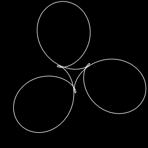
Imagine a lumpy surface which cannot be directly seen because a plate of thin, springy sheet metal lies on top of it. Rivets attach the plate to the underlying surface at random points; otherwise the thin metal sheet more-or-less follows the underlying surface in a manner that minimizes the forces needed for bending.
G’MIC’s rbf command has, for its lot in life, the task of estimating the locations of points on the thin metal sheet, given the placements of a handful of rivets. Unless told otherwise, rbf employs the thin plate spline radial basis function, {r^2}\ln(r) , to establish the likelihood of deflection of a point on the sheet metal in the neighborhood of a rivet, with r>0 , the radial measure of separation. For very small r, regions close to rivets, the likelihood of deflection is minuscule — even negative! — because it is very, very! hard to bend a short scrap of sheet metal. On the other hand, for larger r, the sheet metal accommodates greater deflections.
And so it goes: for most locations, rbf estimates surface positions by assessing the locations of surrounding rivets, all scattered in different directions. In some locations, a nearby rivet dominates; other places may fall under the sway of numerous rivets, some near, others far, none dominating. In all cases, rbf runs with the minimum energy trope. Whatever the position of a given sheet metal point might be, it reflects a ‘minimum energy solution’ — the least deflection needed to obtain that position.
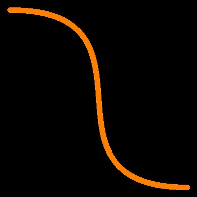
In this setting, the profiles of tracks running along the surface of such thin metal sheets assume lovely curves. They are not cubic, but infinitely differentiable — that is, rates of change, rates of change layered upon rates of change, ad infinitum… may be all smooth curves; cubic smoothness cuts off after the second go. It is simplistic to attach greater aesthetic appeal to infinitely differentialble surfaces, but some find it so — and, in any case, we seek paths orthogonal to the wonted spline(). Away we go.
The heart of ribbons, version two, is splinefun, and at the heart of splinefun is a handful of points — coefficients, now, not rivets — few in number and conjured up from the aether (they were made up). rbf calculates the least energy surface which embeds these coefficients. This calculation produces a two channel image — plotcoords — the minimum energy surface — well, actually, two: one for x coordinates, the other for y. The two minimum energy surfaces furnish parametric arguments for plotting curves on other surfaces: canvases. Mechanics follow.
- Each column of
plotcoords embodies the (x, y) plots of a curve on canvas.
- The width of
plotcoords yields the number of curves. Wider ⇒ more curves.
- The height yields the number of curve data points. Higher ⇒ smoother curves.
- Thickness arises from an imagined calligraphic pen following the curve on
canvas.
That last point recommends further remarks. The pen has a width and an orientation at some angle to the curve’s course. These data allow an offset given by the pen tip’s width and its orientation. The mechanics duplicate curve data points and offsets them. The exigencies of polygon(), G’MIC’s polygon plotter, calls for a sub-path outward and a sub-path back. To meet this necessity, duplicate the curve data set and reverse it, offsetting it by the width and orientation of the pen. These mechanics gives polygon() a closed hull that may be filled by a semi-transparent color. It is uniform, not following from the stamping of semi-transparent shapes at each curve data point, with the collateral overlap of shapes leading to a variation in opacity.
Other matters — calculating the minimum energy surface in a parametric space, then translating such to the canvas, coloring curves in a graduated fashion — are off in the weeds and the details may be drawn from the script. Following, then, are various sets of ribbons plotted in the minimum energy style.
   gmic ccnt=37                                              \
   -input 1024,1024,1,3,lerp([20,17,38],[33,38,46],y/(h-1))  \
   -name canvas                                              \
   (252,233,59^115,22,210^22,210,186)                        \
   -permute. cyzx                                            \
   -resize. $ccnt,1,1,3,3                                    \
   -name palette                                             \
   -splinefun[canvas] [palette],64,3,9,65,1                  \
The above illustrates a few coarse strokes of a broad-tipped pen , 24 pixels, angled at 15°, each stroke at 25% opacity.
Complexity — splinefun’s third parameter, is 5 ⇒ 2^5 = 32 randomly positioned coefficients, which engenders a more complex surface, and, following on, more twisty curves on canvas.
Many very nearly transparent curves gives rise to the illusion of weirdly illuminated surfaces. At the end of the day, we are plotting discrete pixels, like it or not. With closely spaced curves, this reality brings about Moiré patterns.
More transparent curves, following more complicated courses, minimizes — but does not eliminate — such shortcomings. In other approaches, render large, then reduce to small: an anti-aliasing method for those with the memory chips installed.
That’s it for now. Have fun.