Oh interesting! Thanks everyone this is super helpful!
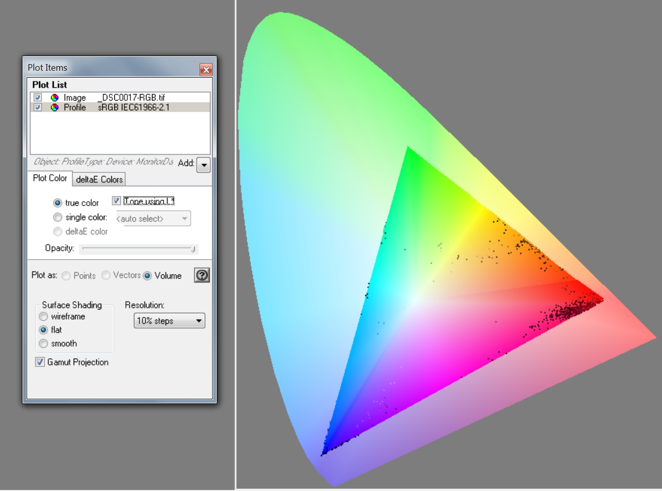
@snibgo, what did you use to make that plot, out of curiosity? @Terry It would be so cool to see pixels plotted relative to the bounds of various color spaces in DT! More or less like the CIE plots shown here. I’ve been wanting to see something like that in order to wrap my head around it and was thinking about breaking out python or matlab/octave to do it haha.
In the interest of really, actually understanding this, let me try to talk through it from the ground up; please correct me where needed. Also, apologies if this is too deep down the rabbit hole, I’m just very interested to learn 
— Deep Dive —
Ok so first, each pixel collects light within a given band (approximately Red, Green, or Blue) and outputs a number from (for the sake of argument) 0 to 1, proportional to the amount of light it collected. Any combination of pixel values at this stage have real physical meaning and so can’t really be outside of the CIE 1931 color space (the horseshoe, as @snibgo put it), even though they aren’t in a well-defined CIE color space yet. Those pixels are then more or less interpolated (demosaiced) in one of a handful of ways, generating single pixels with 3 color channels each (values also between 0 and 1). At this point, there are a number of artifacts that can creep in (aliasing, zippering, etc.), but these are still values that correspond directly to the amount of light received in a certain band, so there can’t really be a combination that is non-physical. The trick, however, is that these RGB values refer to the total amount of light within a certain band, as opposed to what combination of a few very specific primary colors would be required to create the impression of the original color the sensor was exposed to. This is what the input color matrix is doing, but it is not a trivial task because our cones have quite a lot of overlap so it cannot just be a direct mapping.
Now, we would want to map this directly to an independent tri-stimulus space like XYZ or LMS, and this is where imaginary colors can get generated. Ideally, this mapping would be contained within CIE 1931 but any map between these two spaces would have to be based on real-world experiments and so probably requires some interpolation. If that is done by an algorithm rather than a simple LUT, I would guess it’d be optimized for more “common” colors and likely has some distortions at the extremes, which could accidentally bleed into imaginary colors?
— TL;DR —
The implication here is that the fix for the imaginary color problem is to get a better input color matrix that is optimized for more saturated colors (and for my specific camera, for that matter). Would calibrating with a color card do the trick you think?
As for just being outside of any usable color space like rec2020, it seems like it is just normal for a camera’s gamut to be way wider than most useable color spaces so I just need to artificially tweak the colors to get what I want (as @AD4K said), or else just live with the clipping DT does automatically.
— end —
@kofa: yeah, I guess I’ve been worried about it for two reasons: 1) I’m just curious and would like to understand what’s actually happening better and 2) I’m planning to get a print made of some version of this and I’d like to know where the limits of the printer’s profile is so I can get the most vibrance out of it I can. It would be really nice to be able to separate where in the pipeline things are being clipped for both debugging reasons and also in order to get a better handle on #2. I think being able to plot pixels against the color space in question (as @Terry was suggesting) would be super useful for that as well.