A Greedy Algorithm to Paint an Image by Randomly Exploring a Space of Brush Strokes.

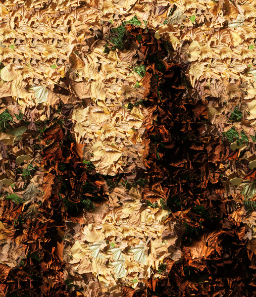
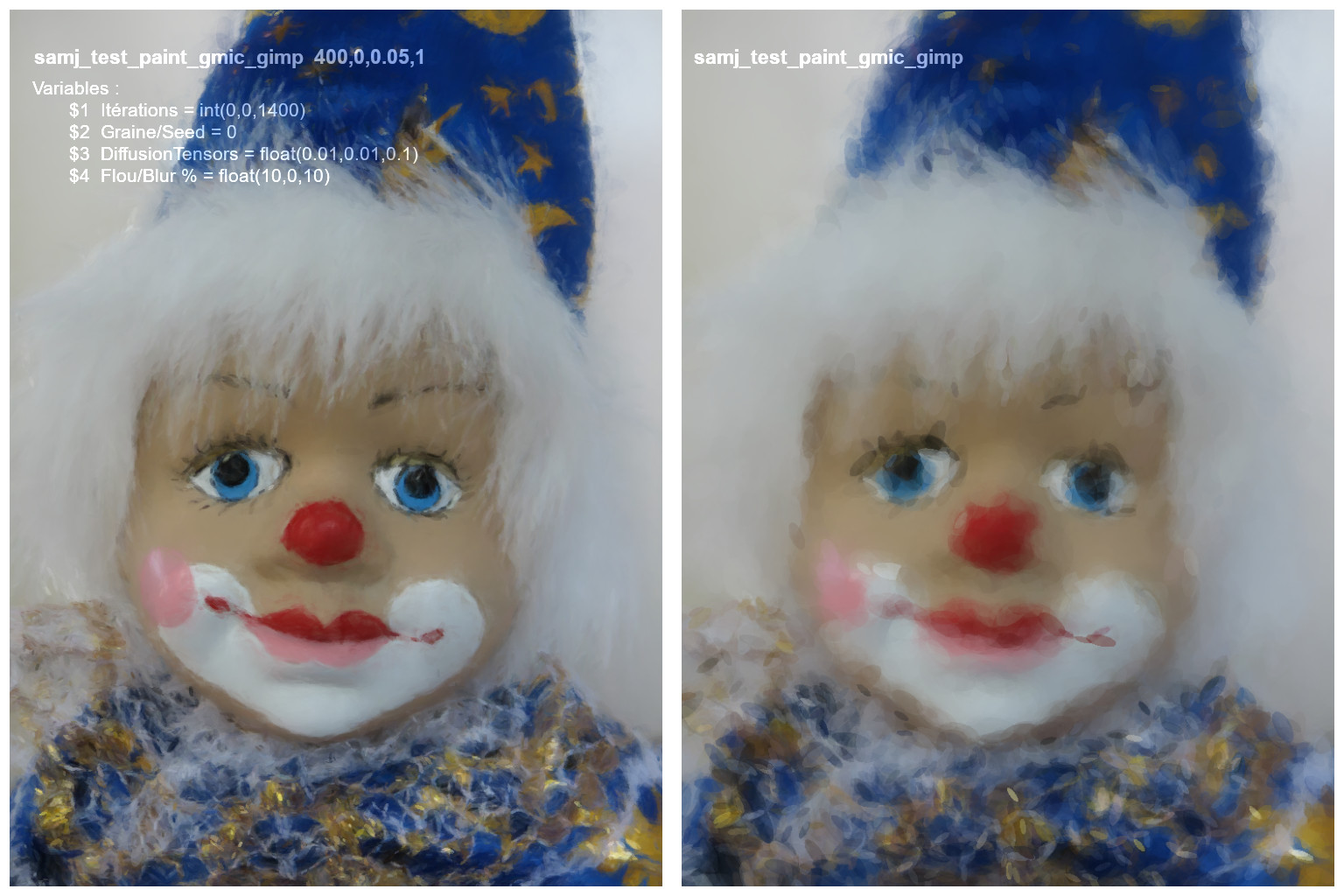
Just had some fun tonight with an idea I wanted to experiment. Basically, the script tries to “paint” random brush strokes on a white canvas, in order to get closer and closer to the input image.

Here is the G’MIC script:

paint :
  100%,100%,1,3,255
  +mse[0,1] mse_best={i[1]} rm.

  repeat inf
    100%,100% noise. {u(0.3)},2 gt. 0 distance. 1 lt. {u(2,20)}% deform. {u(40)} gt. 0
    +label_fg. 0 {iM+1},1,1,3,u(0,255) point. 0,0,0,1,0 map.. . rm.
    +blend[0] .,shapeaverage0
    blend[-2,-1] alpha,{u(0.5,1)}
    distance.. 0 n.. 0,1 pow.. {u(2)} f.. "i?cut(i+u(-0.25,0.25),0,1):i"
    +j[1] .,0,0,0,0,{u(0.7)},..
    +mse[0,-1] mse={i[1]} rm.
    if $mse<$mse_best
      j[1] . mse_best=$mse +e $mse_best
      to. {round($mse_best)},0.01~,0.01~,4%
      w. on. frame.jpg,$>
    fi
    rm[-3--1]
  done

Here is the result (takes a lot of time to render by the way):

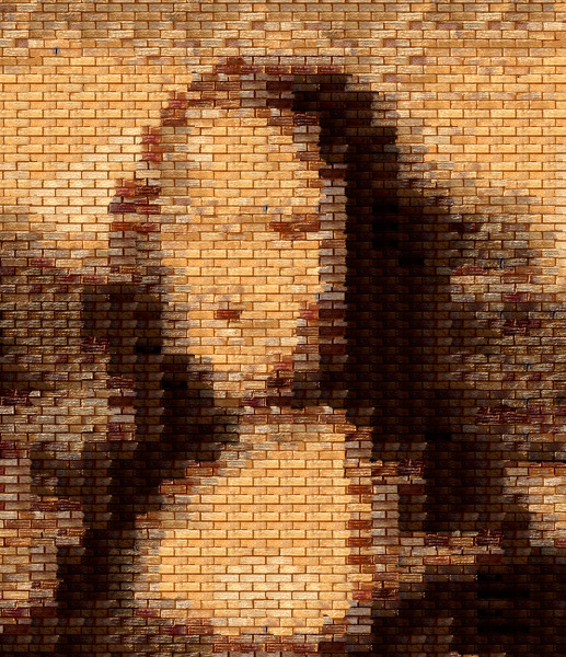
What happens when considering only a “solid” brush ?

11 Likes

I’ve tried to improve the algorithm a little bit tonight, with interesting results.

4 Likes

Very nice!
The first fox has a lovely softness, but perhaps with a look that is too monotonous across the image. One might expect a different look to the strokes in fine detail compared to coarse detail. The second fox appears to do just that, albeit replacing the soft quality with a smudgy one. One could have a lot of fun playing with these. I also really like the solid brush.

Good stuff. Instead of conventional brushes, we can use leaves or bricks, with a much lower resolution:

qlt_monalvs3

qlt_mona_brk

3 Likes

I have had fun doing similar things but I always force stop. My laptop cannot keep up: runs too slow and hot! I do have a slightly newer more powerful machine now but haven’t gotten around to setting it up…

Could you provide the code for that? Always interested in others’ problem solving process.

Still a few improvements :

Here is the code source.
@grosgood may be interested by that, I’m using a lot of diffusion tensors to achieve the painting simulation :slight_smile:

paint :
  +diffusiontensors 0.1,1,0.5,2
  +b[0] 10%

  f=0
  repeat inf,t
    beta={1-exp(-$t/70)}

    100%,100%,1,4
    {u(16,512)},1,1,1,"*
      const da = 10;
      const dl = 1;
      const beta = $beta;
      const bs = lerp(80,2,beta);
      const anisotropy = lerp(0,1,beta);
      lmax = u(lerp(1,20,beta^2));

      X0 = round(u([w#0,h#0]-1));
      RGB = [ I(#0,X0),255 ];

      for (a = 0, a<360, a+=da,
        X = X0;
        U = [ cos(a°), sin(a°) ];
        for (l = 0, l<lmax, l+=dl,
          C = I(#1,X,1);
          T = [ C[0],C[1],C[1],C[2] ];
          eig = eig(T);
          l1 = eig[0];
          l2 = eig[1];
          u = eig[2];
          v = eig[3];
          ellipse(#-1,X[0],X[1],bs,bs*lerp(1,(1 - l1 + l2),anisotropy),atan2(v,u),1,RGB);
          nU = T*U;
          X+=nU*dl;
        );
    );" rm.

    sh. 100% distance. 0 n. 0,1 pow. {u(0.5)} *. 255 rm.

    opac={lerp(0,0.5,$beta)}

    blend[2,-1] alpha,{u(0.15,$opac)}
    w. # on. frame.jpg,$f
    f+=1

  done
4 Likes

As it happens, I am stepping though the pastebin version now. +diffusiontensors being catnip. Alas, may be mute on this topic for a few days, but I have promised playtime for myself this weekend. Which. Does. Approach. Ponderously.

1 Like

This — I find — is the useful bit, in conjunction with tracking orientation, as in the physical effort a painter expends is much in the thought of laying down the brush stroke in ‘just the right way’. The merit function (mse) may also invite creative debauchery, choosing to customize it away from Old School mean square to something more peculiar. Must run now. City calls.

Wow, this one has minimal detail but captures lights and shadow very well for a 3D effect.

I think I’m done now with the prototype for this algorithm.
I’ve tried a lot of different things, and this is what I get at the end:

paint :
  +diffusiontensors 0.01,0.95,0.5,1
  +gradient_norm..
  # +f[0] 255
  +b[0] 10%

  f=0
  repeat inf,t
    beta={1-exp(-$t/100)}

    100%,100%,1,4
    {u(16,512)},1,1,1,"*
      const da = 15;
      const dl = 1;

      const beta = $beta;
      const bs = lerp(60,1,beta);
      const anisotropy = lerp(0.5,1,beta);
      const opac = lerp(0.5,1,beta);

      X0 = round(u([w#0,h#0]-1));
      RGBA = [ lerp(I(#0,X0),u([255,255,255]),0),255 ];
      lmax = lerp(1,10,beta^2);

      for (a = 0, a<360, a+=da,
        X = X0;
        U = [ cos(a°), sin(a°) ];
        for (l = 0, l<lmax, l+=dl,
          C = I(#1,X,1);
          T = [ C[0],C[1],C[1],C[2] ];
          eig = eig(T);
          l1 = eig[0];
          l2 = eig[1];
          u = eig[2];
          v = eig[3];

          RGBA[3] = opac*lerp(10,255,min(1,i(#2,X0)/10));
          nbs = bs;
          nbs*=lerp(3,1,min(1,i(#2,X0)/20));

          ellipse(#-1,X[0],X[1],nbs,nbs*lerp(1,(1 - l1 + l2),anisotropy),atan2(v,u),1,RGBA);
          U = T*U;
          X+=dl*U;
          U/=max(1e-9,norm(U));
        );
    );" rm.

    opac={lerp(0,0.5,$beta)}

    blend[3,-1] alpha,{u(0.05,$opac)}
    w. -1,-1,0
    on. frame.jpg,$f f+=1

  done

Next step would be to convert it to a filter for the G’MIC-Qt plug-in…
If only I had the courage to do it! :smiley: :tired_face:

5 Likes

@David_Tschumperle

Bonjour,
I did some tests on 3 versions of the ‘Paint’ program with a limited number of iterations.
I like the rendering with program 1 at the top of this thread with a more surprising and richer rendering.
Thank you for all this beautiful work.
:o)

2 Likes

This looks like a reverse explosion of the trees, very beautiful :slight_smile:
Thanks for sharing!

That’s a nice one.
As far as I know, the GitHub wiki is the only place where there are development examples for writing a gmic-qt compatible plug in, to wit:

  1. How to create a custom filter in the G’mic plug in
  2. Making better custom filters

The gmic-qt adaptation of this could serve as an illustrative example in a third, grande finale “Making even more interesting custom filters.” It is a robust example and makes use of math expressions in an interesting way.

Possibly there is a place for such a “1. 2. 3.” series in the tutorial conglomerate, a Cookbook, as there is nothing there at the moment which connects G’MIC scripting and writing a gmic-qt filter, though just that task, and no other, is what might likely motivate most (potential) script writers. Probably save further remarks on this for my end-of-month “Tutorial Fragments” write-up.

Merci :o)

https://bloglaurel.com/post/en-vrac-20/1637
1 Like

Bonjour,

It is possible to test the last filter created by David on G’MIC-QT for GIMP 2.10 - 2.9.9_pre
It is necessary to update.
You can place a command in ‘Various> Custom Code’, for example :
samj_test_paint_gmic_gimp 400,0,0.05,1

Variables samj_test_paint_gmic_gimp $1,$2,$3,$4
$1 Itérations = int(0,0,1400)
$2 Graine/Seed = 0
$3 DiffusionTensors = float(0.01,0.01,0.1)
$4 Flou/Blur % = float(10,0,10)

There is no GUI because it’s a test.

2 examples:

Still working on this painting algorithm, and many changes have been made so far.
Hopefully, it will become a usable filter for the G’MIC-Qt plug-in soon :slight_smile:

1 Like

@David_Tschumperle
Bonjour,
Thank you, It’s very appreciated and very nice of you to create this new filter.
:o)

I love this!

(is there any handholding guide to create render animations like those here? I love them and want to try them on some of my pics!)

2 Likes

@johnny-bit

Bonjour
Do you want to create a video when using the filter (sample paint_3_test.mp4) ?

If this is the case the frames saved during the operation of the filter under ‘GMIC-QT-GIMP Win’ must be in .png format.

1 Like