So, before we get started with the rotations, a bit about the “Notorious 6” (for their friends, just “N6”) and hue preservation.
The term “Notorious 6” is used to describe the phenomenon that per-channel application of (monotonically increasing) curves leads to all colours tending to one of the 3 primaries or 3 secondaries, causing unnaturally yellow sunsets etc.
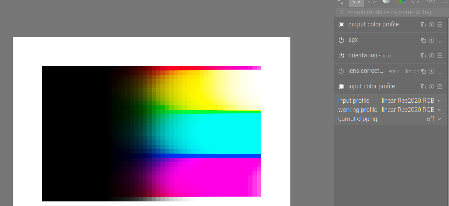
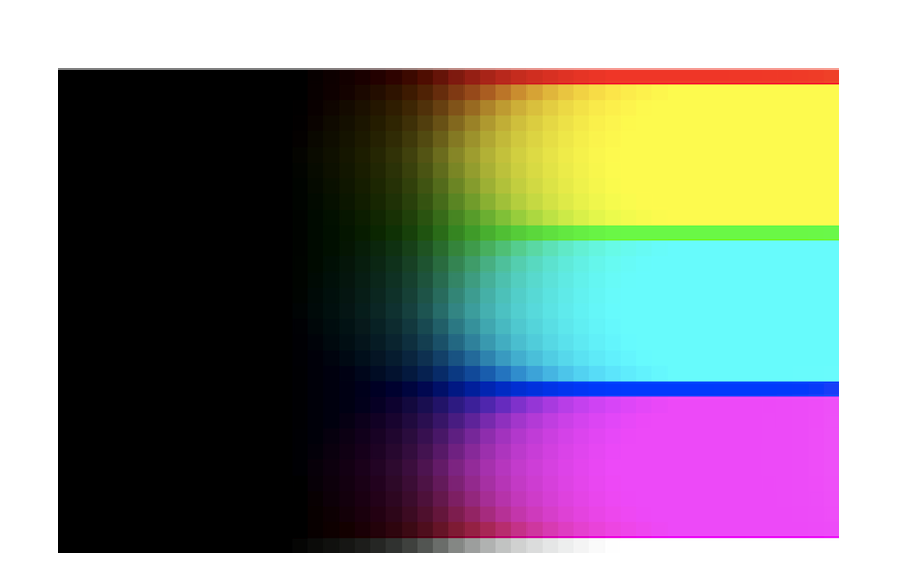
Download this image, and open it in darktable: Testing_Imagery/RGB_sweep_smooth_31x50.exr at main · sobotka/Testing_Imagery · GitHub
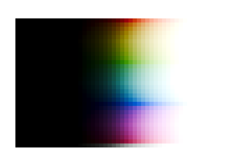
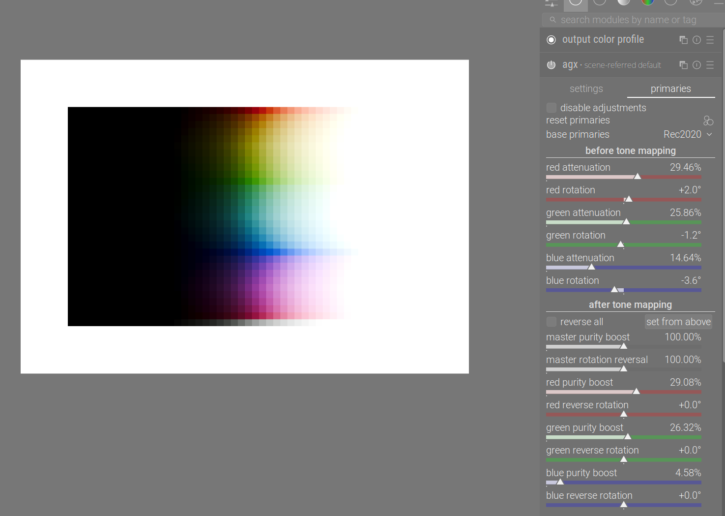
Once opened in darktable, with agx using the scene-referred default, blender-like or smooth preset (each gives a different, but fundamentally similar result):
So where are the N6?
Well, disable the primaries altogether:
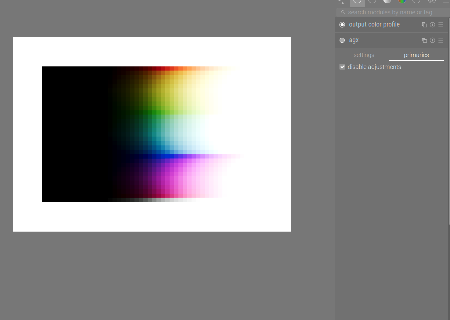
We can now start to see there’s only a red row, with most of the area under it turning yellow, then a bit of red, then some cyan, then a blue, and then quite a bit of magenta.
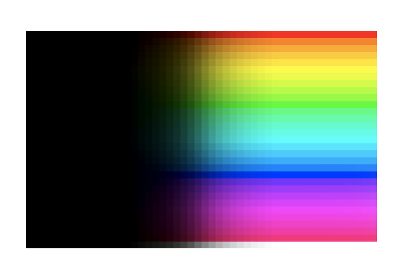
But the actual horror is yet to come. The input image is in linear Rec 709. Processing in Rec 2020, a larger space, means the colours, as far as Rec 2020 is concerned, are not fully saturated (in a way, it’s as if some desaturation had been performed via attenuation of the primaries – consult the Rec 2020 to sRGB example in the previous post). So, either set the input profile manually to Rec 2020:
Or leave it as embedded matrix, and load the unmodified primaries, and set the base space to sRGB:
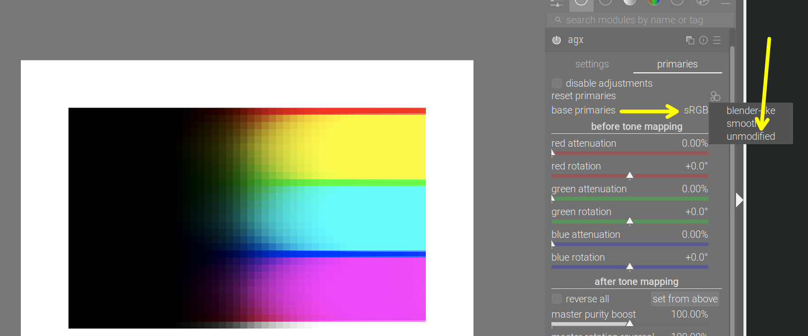
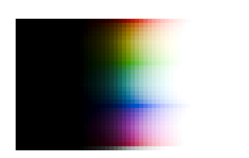
The six horsemen have just arrived. No nice path to white, and most bright colours have collapsed into the secondaries, save for the pure primaries.
What’s going on?
Let’s fire up the tool again (I’ve enhanced it with more direct RGB and hue display).
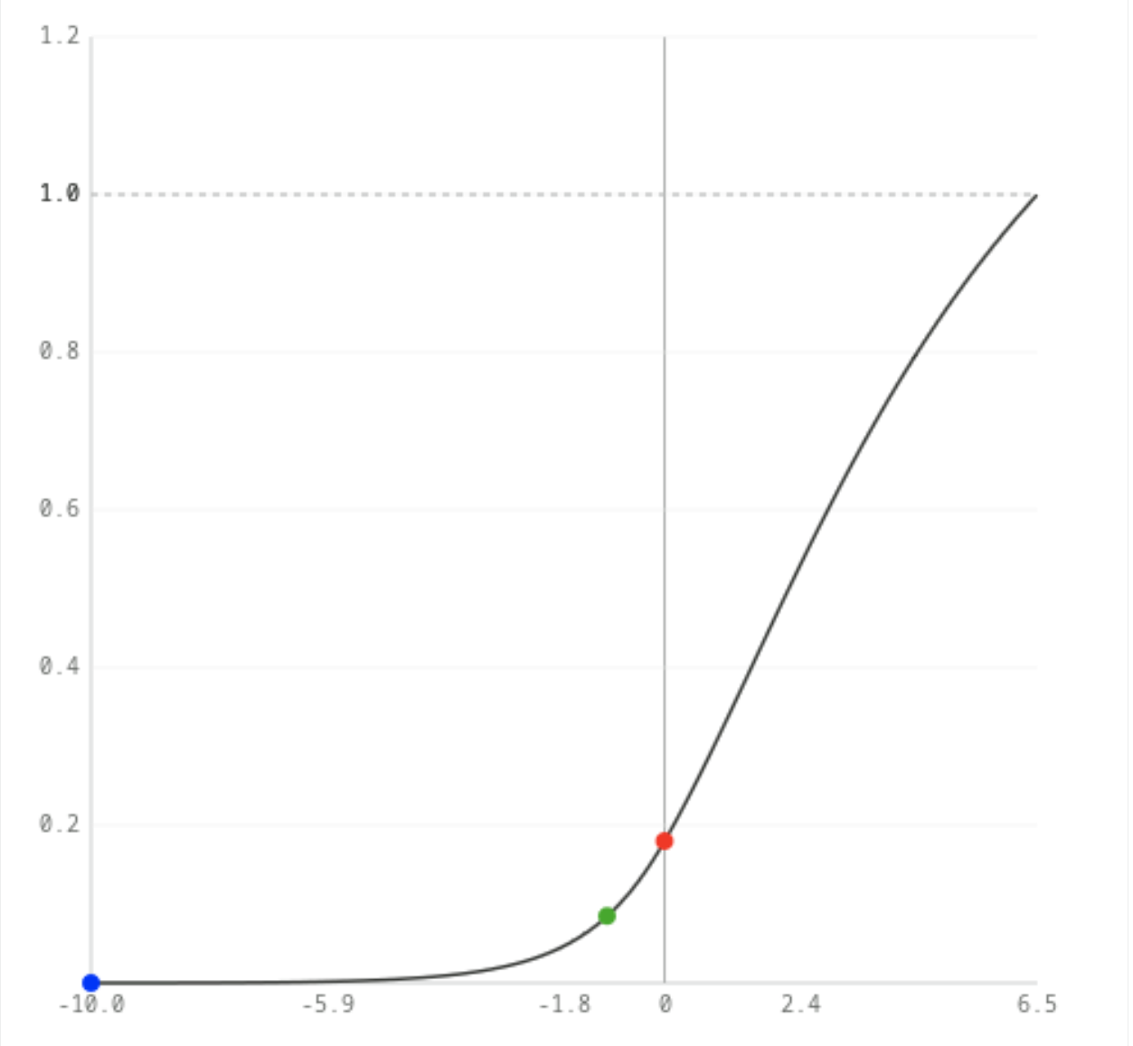
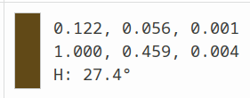
We’ll start with a fully saturated colour. Again, ‘fully saturated’ means ‘at least one component is 0’. We’ve already seen that without primaries adjustments, primaries just remain primaries, so we’ll use the colour (0.18, 0.09, 0). This will give us a starting hue angle of 30°, orange (red is 0°, yellow is 60˚, green is 120°, cyan is 180°, blue is 240°, magenta is 300°).
This will be more or less preserved. Using the new hue outputs displayed above the chart:
Tone curve (log → gamma encoded)
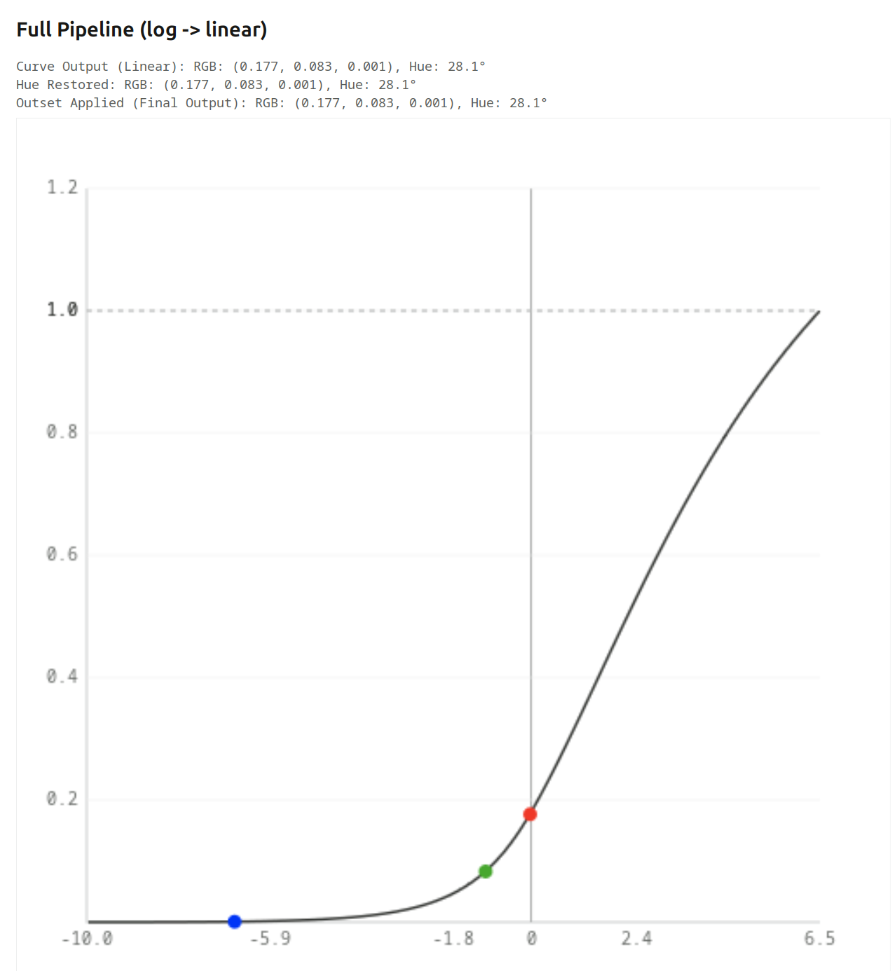
Inset Applied (curve input): RGB: (0.180, 0.090, 0.000), Hue: 30.0°
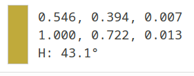
Log Mapped: RGB: (0.606, 0.545, 0.000), Hue: 54.0°
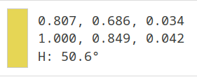
Curve Output (Pre-Gamma): RGB: (0.459, 0.326, -0.000), Hue: 42.6°
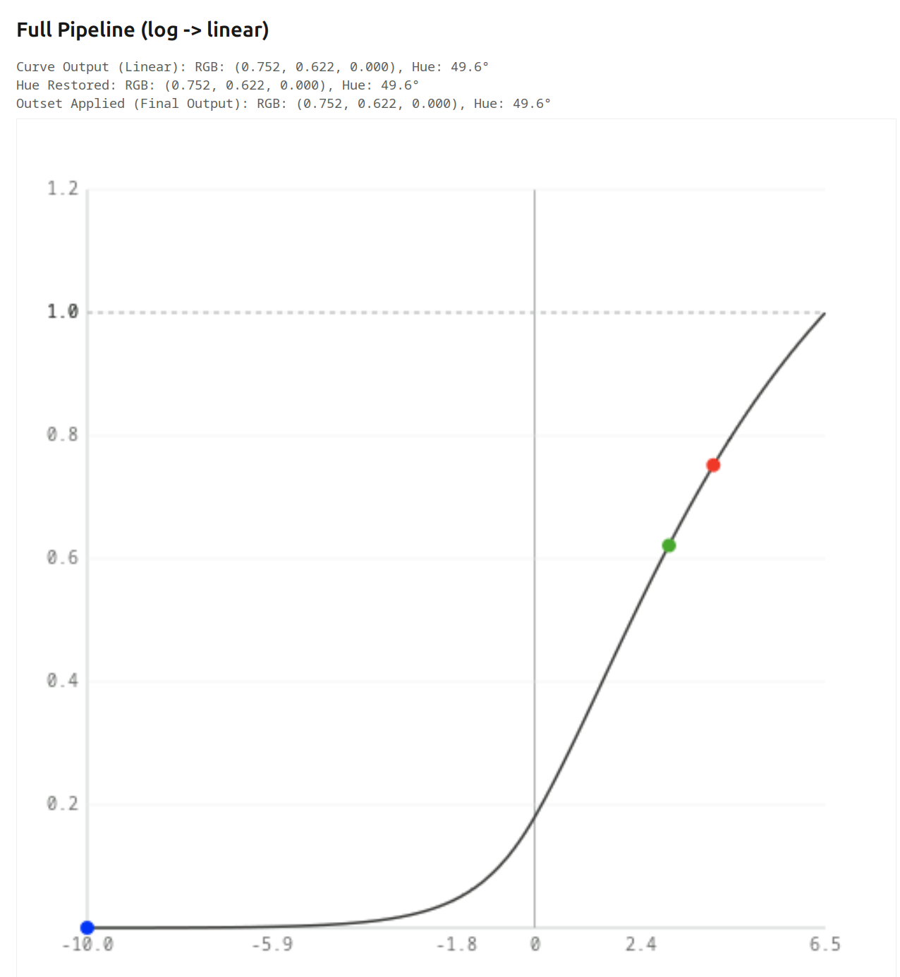
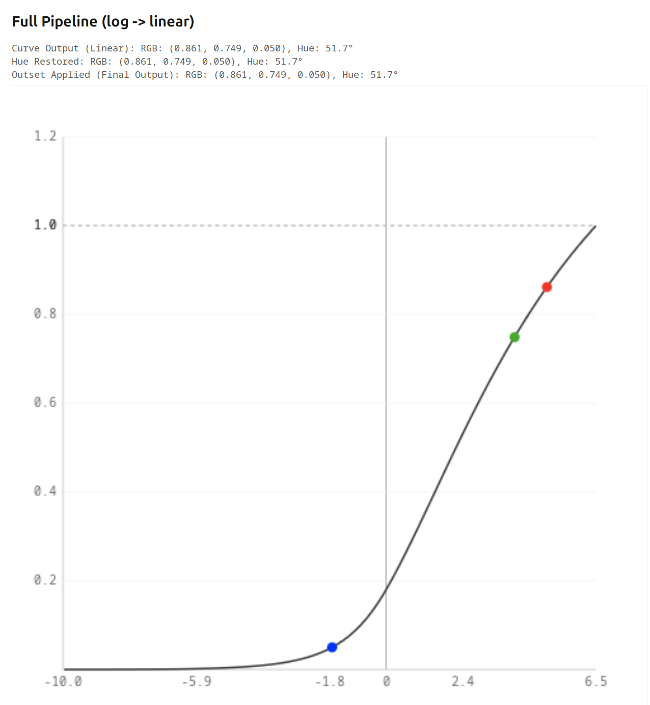
Full Pipeline (log → linear)
Curve Output (Linear): RGB: (0.180, 0.085, 0.000), Hue: 28.3°
Hue Restored: RGB: (0.180, 0.085, 0.000), Hue: 28.3°
Outset Applied (Final Output): RGB: (0.180, 0.085, 0.000), Hue: 28.3°
We don’t use an inset, so of course Inset Applied still shows 30°, but what happens afterwards?
Log strongly compresses values. From a ratio of 2:1 (18% red, 9% green), we go to 2:1.8 (60.6% red,54.5% green), and the hue shifts almost to yellow (54.0°, yellow is at 60°).
Then, we have the tone curve, which adds contrast, and pulls those a bit apart, red at 45.9%, green at 32.6%, hue at 42.6°. (You can read the radios from the table, I did not add them above the charts.)
Then, we get the linearisation, which pulls the values further apart; we have no hue restoration or outset, so the final result is red: 18%, green: 8.5%, hue: 28.3°.
The log → linear graph looks like this:
However, increasing the the exposure slider will push the x-coordinates to the right. Initially, as we saw, the red component (in the output) is almost twice as large as the green (close to the original 2:1 ratio), as we push exposure, the linear y ratio drops quickly, and the hue shifts (look at the output (y) red to green ratio, not the difference!)
+2 EV

+4 EV
As we go higher, and the curve starts to lose contrast (slope is reduced), even the difference starts to drop, and the red:green ratio drops even quicker:
+6 EV

Finally, once red goes into saturation, increasing exposure only pushes green. +6.5 EV, 7 EV, 8 EV:

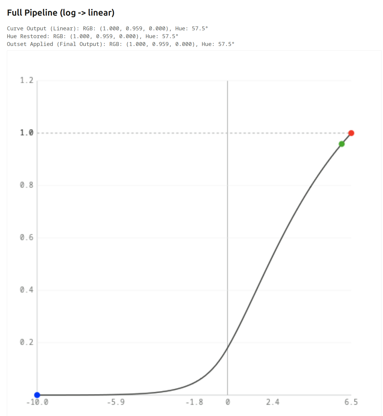
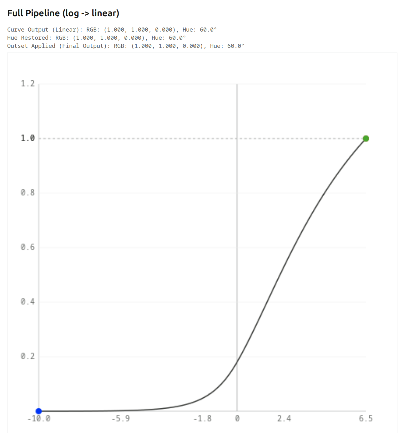
At that point, red = green, so we get yellow.
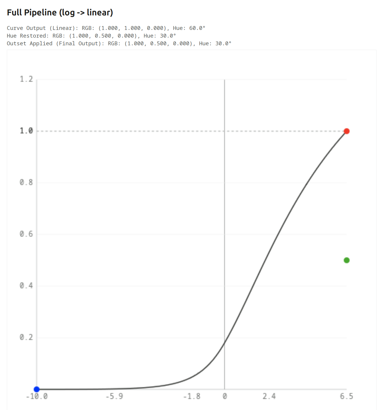
This is the kind of skew that hue preservation corrects: it records the hue angle after the initial primaries manipulations, and re-applies it before the final primaries changes. It is only designed to counter the skew caused by the log mapping + tone curve + linearisation.
Turning it on full-force for the final image, we can see green gets pushed down to 0.5, restoring the original 2:1 ratio (it works the same at the other exposure levels, too):
What happens if the colour is not fully saturated?
As long as the 3rd component is much lower than the other two (so the colour is quite saturated), we get more or less the same (this is without hue preservation, again):
We get a mixture of desaturation and hue shift. Output samples at some exposure levels:
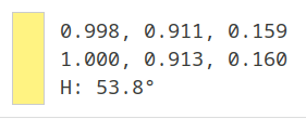
And if the 3rd component is similar in value to the other two (initial hue angle: 20°)):
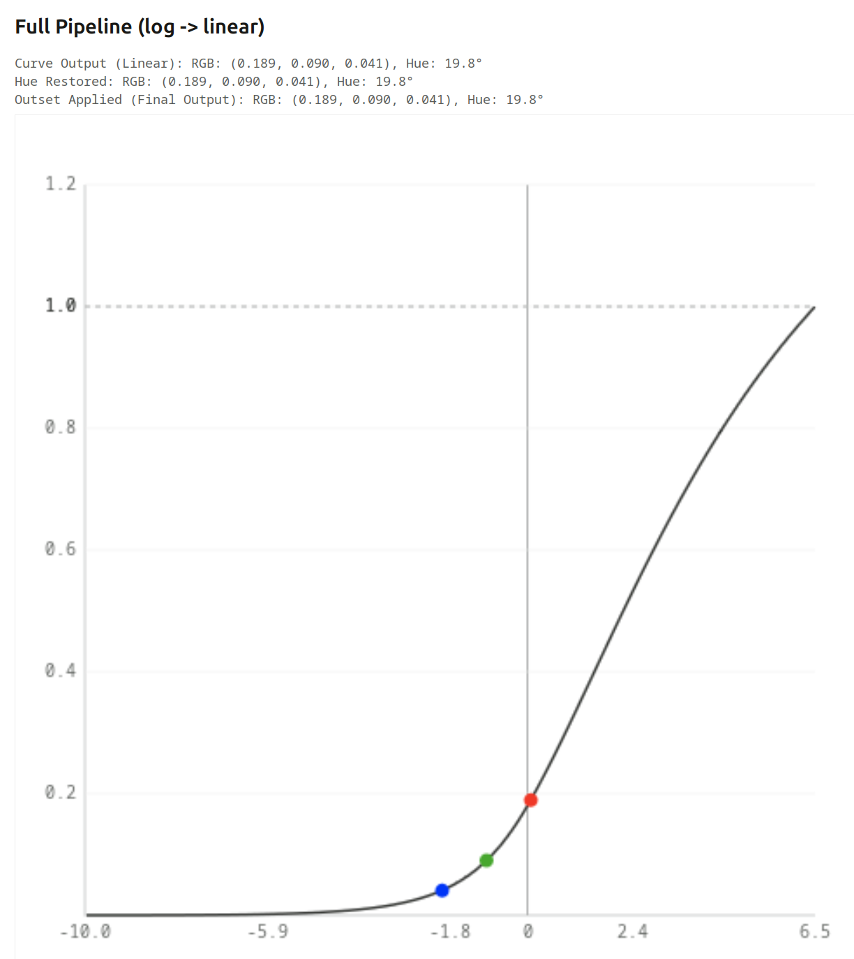
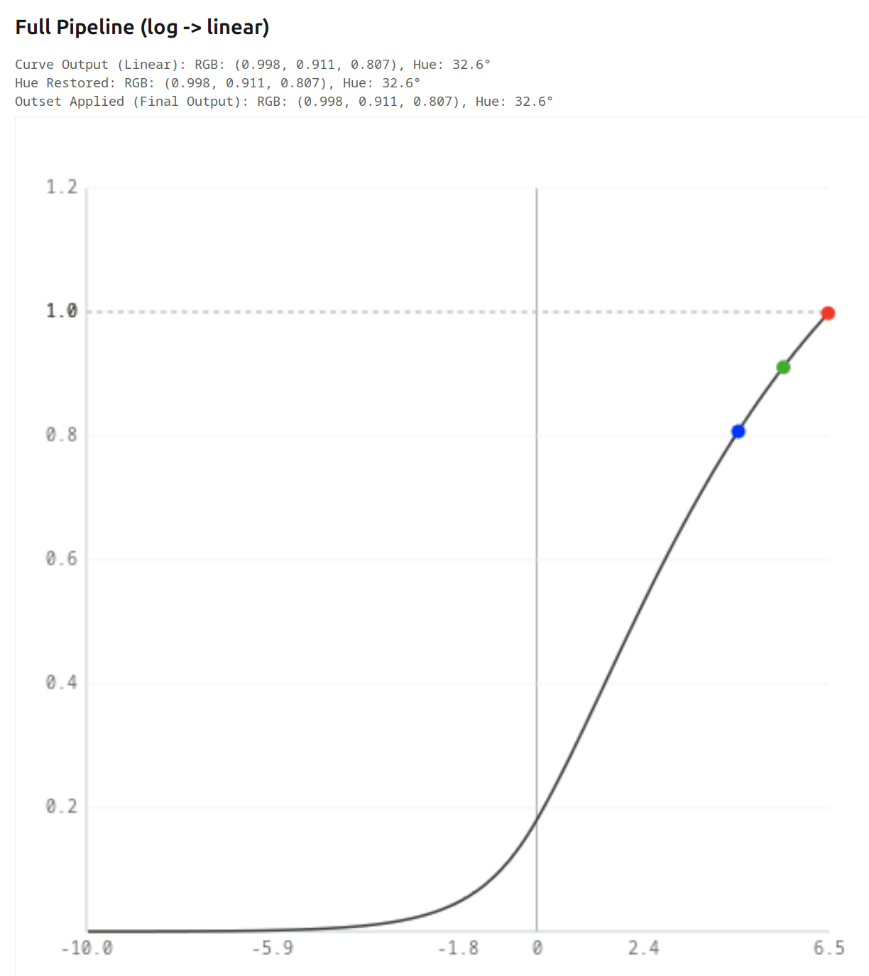
Table (final output):
Note that without attenuation you lose the path to white, and hue preservation will of course not correct that.
No attenuation without / with hue preservation:
Brightness is also affected, that’s due to the simple HSV algorithm. I can try replacing it with something more sophisticated, but since agx is normally used with proper primaries, it may not be important.
The scene-referred default preset, without/with hue preservation: