The key word is drop-in, as in “I won’t get the same result with just exchanging one of filmic/sigmoid/AgX for another one of that group” (even after adjusting the parameters for each). Of course, you’ll only use one at any given moment…
If I change the tone mapper, I expect to make changes elsewhere in the pipeline. With that in mind, comparing just the effect of AgX vs. filmic or sigmoid is a bit an over-simplification.
Of course you want to know that. But see above…
And I don’t think @kofa expects to just replace filmic with AgX, with no further changes (the original version wouldn’t allow that anyway, as the module didn’t keep middle gray invariant).
But more likely I would switch to RawTherapee, because there are more tools than just a tonemapper, WB and exposure.
I think the AgX module isn’t there for replacing darktable but just to give more options for tonemapping respectively handling difficult light situations. So why should I try to avoid local contrast or any other module?
@Soupy I appreciate your deep dive into the different approaches but I have to disagree with removing Slope, Offset and Power for a number of reasons.
The Look control functions provide a quick and easy way to frame the image and provide a good starting point for additional edits. For a lot of users the entire Look section may be enough. They also address a common complaint with new users who are looking for a way to quickly replicate the SOOC jpeg look, so this is a good way for inexperienced users to start off with Darktable.
There are also fundamental differences between Look and Sigmoid, where Slope and Offset work across the entire dynamic range while Sigmoid Black/White relative exposure pivot around the mid grey point. These differences are not redundant - they compliment one another.
Also, there is no analogous function to Power that is found below in the Sigmoid section, and that is a feature is extremely useful in shaping the tone at the start as @s7habo has demonstrated that above. Yes, you could do something similar in the Color Balance RGB 4 ways tab, but its simply convenient and well placed here in AgX.
More importantly, the White relative exposure exhibits anomalous behavior if pushed too hard and there’s a point where the shoulder power becomes inoperative. Perhaps that might be corrected later, but you don’t have that problem right now if you begin with SOP. So as it stands right now, I can’t use the relative exposure sliders in the way you want to use them.
I think the way that @kofa (correction: @MStraeten)has laid out the module is brilliant with the collapsible Sigmoid and advanced options. Personally, I start at the top with SOP and work my way down and this layout is every efficient for me. But it also leaves the options for users who have their own preferred approaches.
I second that and well most of what you note about the module. I think having them there should let people play to the extent they want and they can also add those functions to a QA panel whereas if you remove them they could not and in the current configuration the extra functionality is not in the way of the primary module controls… just my opinion of course
I do get it as well and even last night checking in on the terminal window I thought it was hung as it paused for a long time and then it continued and built so I have no idea…I think it has been like that since the first time a did a build…
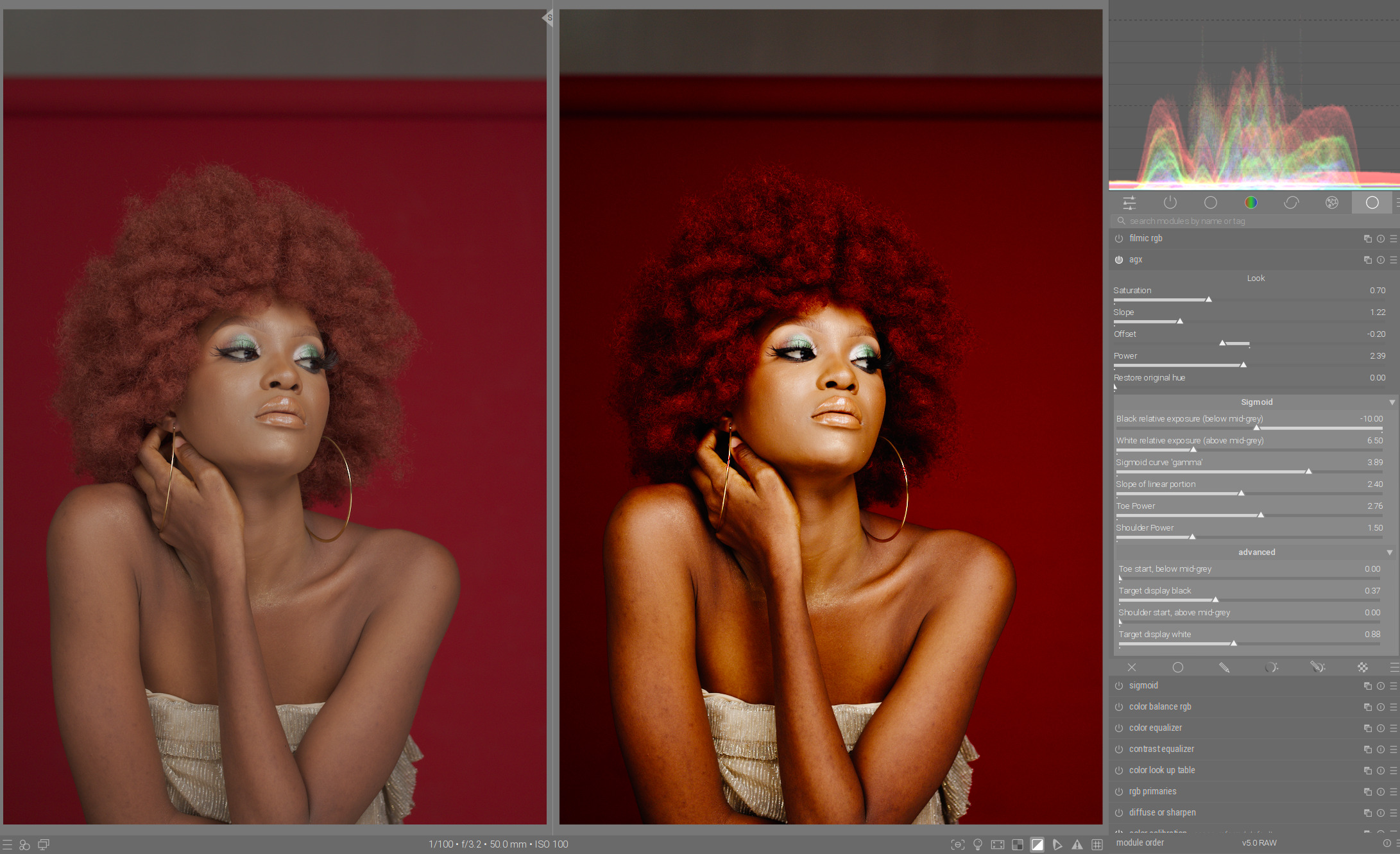
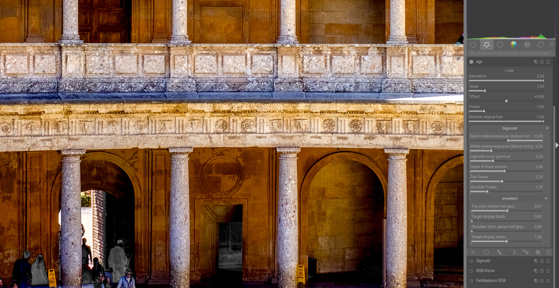
Here I have found a nice example where you can achieve extreme contrasts in medium gray and use target display black/white to keep the black/white point in check to achieve an analog film look:
If I build using ninja instead of makefiles I don’t get those errors, but it does open the script file (tools/generate_styles_string.sh) in wordpad. I close wordpad and it builds just fine. The script generates a list of strings for translation, so if it doesn’t run it doesn’t effect the output.
Like you, my workflow so far is to use the Look controls, then refine with the Sigmoid controls. So, both sections are used. But there is feedback and discussion around doing everything with the Look controls or everything with the Sigmoid controls, in which case only one section is used.
So, I think two basic workflows are starting to take shape:
1: Use Look section AND Sigmoid section
2: Use Look section OR Sigmoid section
I’m not sure we actually need to choose between these two approaches, because the module is flexible enough to allow for both workflows. But I’d be interested to know if there will be more of a “recommended” workflow that the module is designed around or that the manual will encourage for new users. Still early days of course, but just throwing it out there for discussion.
When I was using the initial v1 of this presented by @kofa I was quickly doing one of two things…as already mentioned by @s7habo you could select the punchy preset and add exposure and often have a really decent starting point…but not universally of course and so I found I was using agx to manage teh highlights and then the other controls slope and power to create almost a log like image with room on both sides of the wave form and then I would use RBG CB to target it…likely because I was also very used to using that module. But using the “log” like looking base I found let me apply a wide range of adjustments in the CB module such that I was not only getting a nice final product but discovering several possible pathways to a end point along the way… I could see sticking to this sort of thing and only resorting to the curve tweaking if I couldn’t get where I wanted without it… but truthfully I need way more practice once things firm up to decide and even then it might be image to image what route I would go…
It is subjective, definitely. My point, which perhaps wasn’t clearly made, was not for everyone to compare their results with mine, rather to showcase a new workflow, allowing others to compare the results achieved with it to the one they were already using. In comparing different ways of working, we can learn new things and find the most effective way to use the module, and it is so easy to compare results with the snapshot tool. But apparently no one is interested in doing that, and instead gave a lot of push back. I’ve no idea why.
I never said anyone should avoid that in their workflow as a whole, but in order to understand a single module on it’s own, it’s best to see what its capable of without other modules (aside from the basic necessary modules, of course…).
It’s a thread about agx, and apparently it’s not ok for me to talk about filmic even when asked about it directly, but it is ok for everyone else to talk about local contrast, etc… I personally don’t have a problem discussing these other modules and how they relate to agx, I just don’t get the response I received. I’m actually trying to focus the conversation on the module at hand.
In my workflow I set exposure and white balance, then the tone mapper, before doing creative changes with other modules. Thus, I want the image looking as good as possible using the tone mapper first, thus I want to know how to get the most out of it, before bringing other modules like local contrast in.
I’m happy for people to disagree, I just wonder if they have compared the merits of a different approach? Is the disagreement purely theoretical, or based on observation? Did they try multiple different approaches on multiple images before reaching a conclusion of what they liked best? Do new approaches just get dismissed out of hand? It probably varies by user.
Yes, simplicity is a worthy consideration. I addressed that in my post, and is why I compared the ‘simple’ slope/offset/power approach with what some would consider the more ‘complex’ white/black relative approach, and actually found the latter more simple.
The complexity really arises from having two different approaches that can be used, and users having to choose between them, perhaps without understanding what each function does. Of course if no consensus on ‘best workflow’ can be reached, then there is no way around it, and all the different functions must remain, at the cost of simplicity. This doesn’t effect me personally, I can use it whether simple or complex, was just showing that one’s idea of ‘simple’ might not be ‘simplest’ or even ‘best’.
I agree that’s an important consideration. In the few images I saw this happen, I increased the white relative slider (reducing contrast in highlights) to the point the shoulder power became operable and I could increase it. To me, the result was not any better than simply leaving the white relative slider where it was to begin with, making it a non-issue, but perhaps one can find an example where it would be.
I have heavily tested - not only one workflow. And I tested again, after you pointed in that direction. Anyway, I was not able to get the same pleasing results without the sliders offset power and slope. Have you tried to get a similar result as in this render, without these sliders?
I tried and at least I had no success.
Regarding workflow, for me speed is a very important factor.
So on the most edits I don’t even want to think about the tonemapper it is there but without having adjusted it separately. Therefore, I have a style with different modules including tonemapper settings which I initially apply on every picture. In Ideal cases I don’t have to do more than adjust exposure, and I’m done.
With more complex light situations, there comes need for further editing, but touching the tonemapper is only necessary for round about 10 % of my pictures.
This described workflow is what I do actually with sigmoid. I aim to do it the same way with AgX. I don’t want to use different tone mappers for different things, that’s why I like AgX. It is very mighty but with just the few “look” sliders I can cover most pictures I have. And for the more difficult things, I can use the whole range of sliders to make them the way I want.
On sigmoid I had pictures where it took quite a while until I had the highlights the way I wanted, and I often needed more than just one extra module and masking and so on. With AgX I get much quicker to pleasing highlights. without masking, without extra modules.
But as I told you, this is something I don’t want to do very often and the less modules, the less sliders I need, the faster I am. But that doesn’t mean that I want to have less sliders, if that means less functionality and more time to get to my goal.
So the layout AgX at the moment offers is nearly perfectly fitting my needs.
I can work on a basic setting for my base style. For the more complicated cases I have a few (look) sliders which are enough for most of the rest and the sigmoid section for the really tough ones. And the advanced section for the extremely rare special cases.
I’m looking into these reports of the black and white points breaking the toe and shoulder. So far, I’ve only done the shoulder. So far, I haven’t found a bug; in fact, I confirmed that the shoulder code works as expected. I’ll look into the crushed blacks from @Popanz later, it may be similar, or it may be a bug.
@Dave22152 , since this is useful info for others, I’m replying here. Hope that’s OK.
Long post and a bit of maths follows.
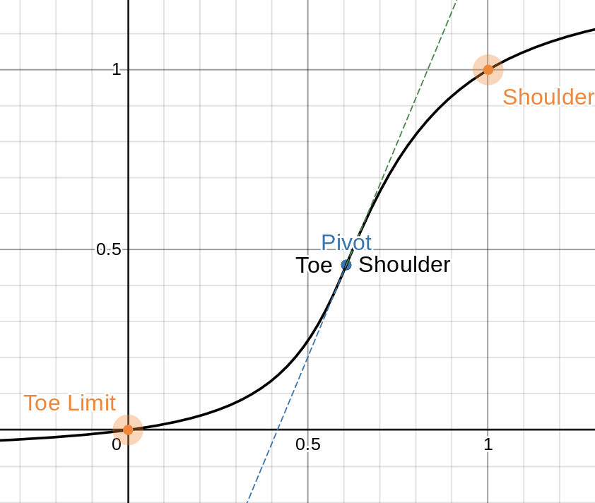
Let me first explain where the ‘mid grey’ is on the plots below:
you specify an exposure range; by default, -10EV … +6.5 EV, or 16.5 EV in length;
internally, the x axis runs from 0 to 1;
0 will correspond to the black point, 1 to the white point
the x coordinate of the mid grey simply splits that range in the ratio (black relative exposure absolute value) : (white relative exposure), for example, 10:6.5. So, with the defaults, the x value of mid grey is 10 / 16.5 (it’s 10 EV above black, on a total range of 16.5), or about 0.6061.
the y value of mid grey, unless you change the default gamma of 2.2, is simply 0.18^(1/2.2), or about 0.4587.
With the default settings, the curve looks like this (Power(P) Sigmoid | Desmos) - the ‘Pivot’ is mid-grey:
Next, we have the slope of the linear range, by default 2.4.
If you use a ‘dynamic range’ that is not 16.5 EV, it gets scaled, so observed contrast (difference of y outputs, given 1 EV of change on the x axis) remains the same. This is needed, because for a larger black/white exposure difference (range), the same smaller x change we have for 1 EV of input change. Therefore, the larger the dynamic range, the higher the slope becomes on the 0 … 1 scale; the lower the dynamic range, the lower the slope.
The range is 13 EV. The slope (user input: 2.4) is scaled to keep the same observed contrast (y change per input EV change): effective_slope = 2.4 / 16.5 * range = 1.89.
The x value of the mid-grey is: black relative exposure / range = 10/13 = 0.769. X distance between mid-grey(=0.769) and white(=1): 0.231.
Y change, if we kept the linear slope all the way to white(x = 1): x-distance * effective_slope = 0.231 * 1.89 = 0.43659.
Y value at x=1, if starting from mid-grey(y=0.4587, see the first section and gamma 2.2) + Y change(=0.43659) = 0.89529. Input white is no longer mapped to output white! Observe the straight line intersecting x=1 at about 0.9:
If you lower the relative white exposure too much, that upward-bending ‘shoulder’ can become extremely steep. The same goes for the toe, in the reverse direction.
If you run darktable from the command line, you can see it outputs a bunch of text:
Because of parallel computation of the editor window and the navigation thumbnail, you may get interleaved, duplicate output; just copy both, run it through sort log.txt|uniq, remove the non-numeric lines, then copy and paste into desmos.
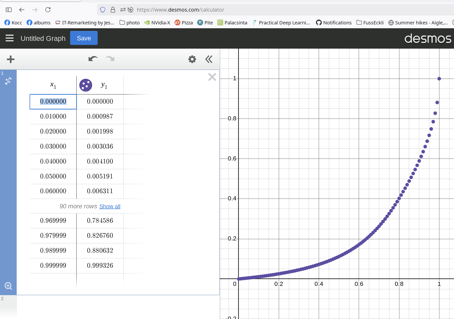
The line need_convex_toe: 0, need_concave_shoulder: 0 tells you if the toe or the shoulder was switched to this workaround mode (0 means no, 1 means yes). The table below is the curve; you can copy the numbers, and paste them into Desmos | Graphing Calculator - here, showing the default settings:
Still with the default settings, but white relative exposure set to 3.72 (-> mid-grey shifted closed to x = 1, range reduced, so linear slope also reduced), the plot is like this – the linear section is just enough to reach white, there is no place for a convex shoulder:
You can see it has become extremely steep, jumping from (0.999900, 0.521533) to (1, 1) .
But there is nothing wrong with the maths: we’ve asked for the white relative exposure to be at 0.1 above the mid-grey, which means that for a change of 0.1 EV in the input, we want the output to go from 0.18 to 1.
If black relative exposure is set to -10 EV, white to 0.1 EV, then the x range of 0…1 corresponds to the exposure range -10 … 0.1, a length of 10.1. This means the 0.18 mid-grey point is 100 times more distant from black (-10 EV, or 0) than to white (+0.1 EV, or 1), its x value is 100/101 = ~ 0.990099.
So, we just told the algorithm to create a curve that goes passes through mid grey (0.990099, 0.45866), and also white (1,1). It did.
So, I hope that answers Dave’s question. If you have a particular image where this explanation does not match the observed behaviour, please let me know.
Now off to check @Popanz 's crushed, blackened toes.
That’s a very detailed explanation . Thank You.
Even so I did not understood everything, I definitely understand now more of the mathematics behind. And using this
helps a lot to understand what the sliders do and what problems can occur.
Yep. Try Power(P) Sigmoid | Desmos.
It does not apply the slope scaling, you have to apply that manually, and it is not aware of the gamma (but you can specify the pivot x, y, so again, you can enter it manually). I may make a version that does those, too.