Solving dynamic range problems in a linear way

anon41087856 · September 12, 2018, 11:37pm

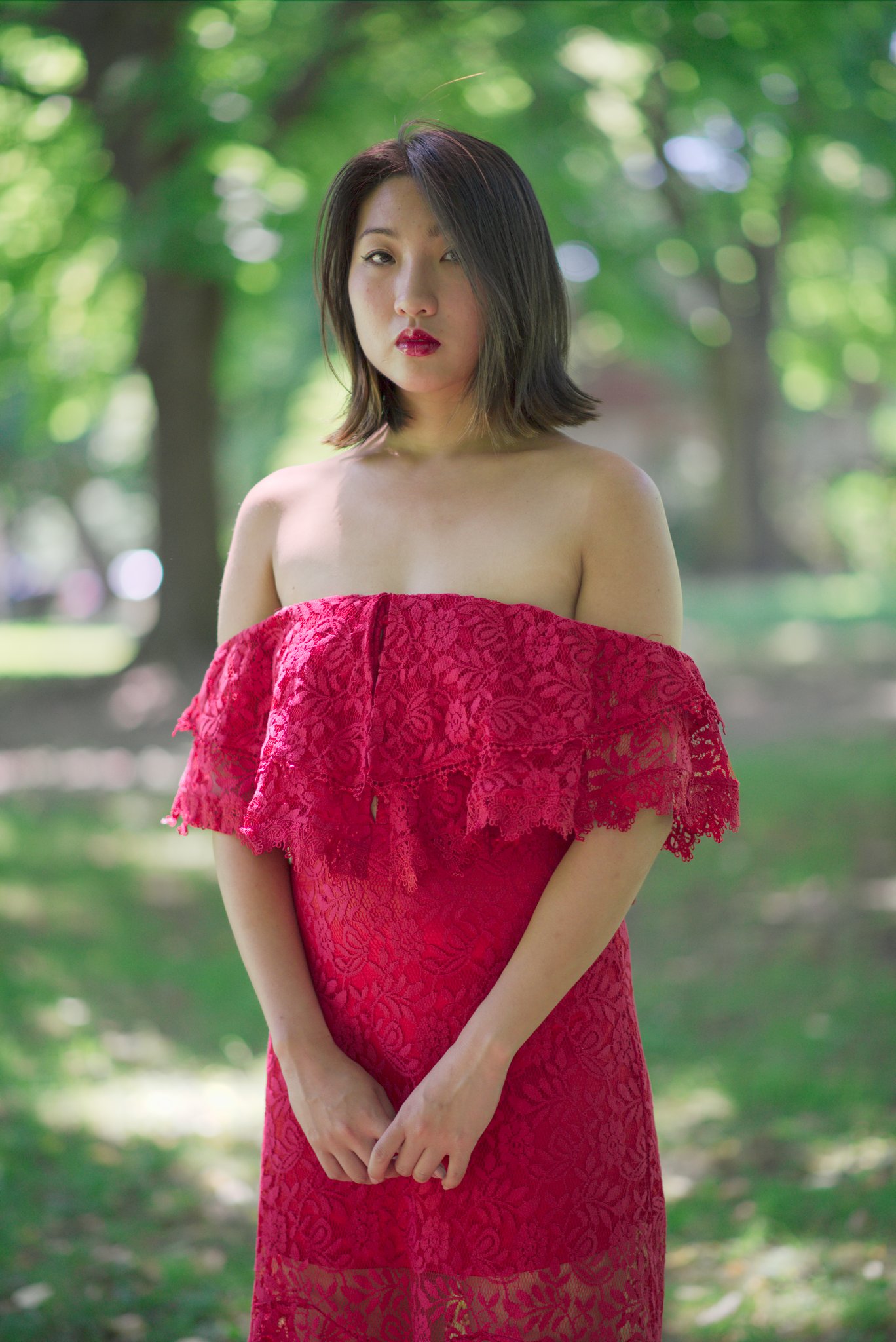
Let’s open this image in darktable:

Here, we have 9 EV of dynamic range, but no overexposed area. How to recover that ?

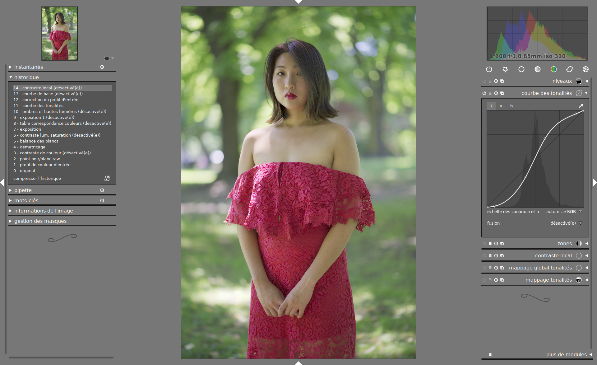
The first option would be to use the input profile correction module and tweak the gamma ( = 0.448) and linear (= 0.05), since we have a custion matrix. Then add a stiff S curve in RGB mode to restore the contrast and saturation:

Well, that recovered the mid-tones, for sure, but blown away some of the highlights and lost the texture of them (look how flat the right shoulder looks). With this module, you always have to sacrifice something, it’s really hard to control accurately what happens from the shadows to the highlights. So now, let’s try with the base curve module instead, to get more control:

It’s better, and we don’t need an additionnal S curve, but see how we still got the highlights burned a little bit ? Moreover, we had to fine tune every control point, which is annoying. Wanna use the highlights/shadows module to fix the highlights ?

Congrats, you just made the subject darker and flatten the shapes ! Using the tonemapping modules will mess you colors even more. So, is there a solution ?

Yes ! This : ASC CDL - Wikipedia, as showed there:

So, i rewrote the input color profile correction in darktable to use this method instead: GitHub - aurelienpierre/darktable at color-grading

Now, back to darktable, the first step is to make the image linear (and very dull):

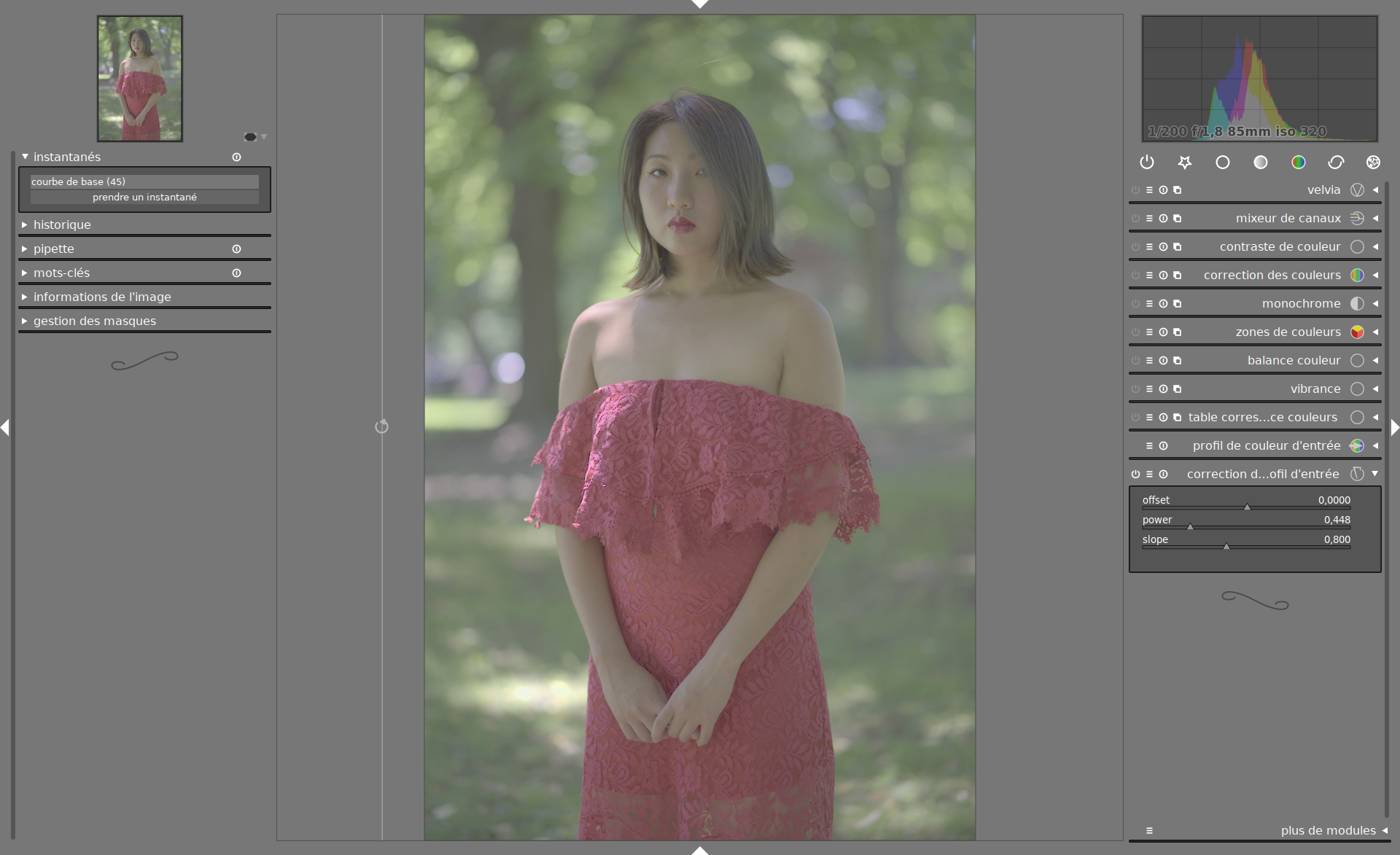
Adjust the slope so than you don’t get blown highlights, then adjust the power (which is essentially the gamma) so that you center the histogram in log preview, and finally, tweak the offset to add a bit more depth in the shadows.

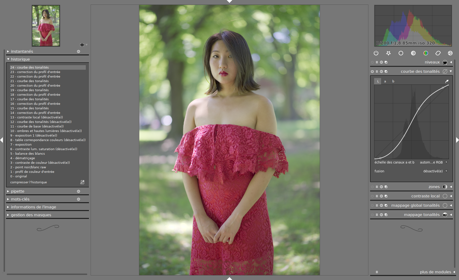
Then, add a stiff S curve in the tone curve module in auto RGB mode:

Final result with hue adjustment (to rewove the green cast from the leaves reflection), local contrast (defaut setting) and Kodak Ektar like profile:

It use to take me ages and never-ending modules stacks to achieve a worse result than that in this kind of setup, especially because the dress color is on the edge of the sRGB gamut. Notice how the highlights are smothly blended with the rest, in the bokeh, without rings or fringes.

Now, you have a reproductible workflow involving 2 modules : 3 sliders to set and 4 control points to set an S curve. I find it easier and quicker to set, more forgiving than the former gamma version (although you could fine-tune it for yours to get close results). It’s beautiful, natural looking, and you don’t get weird color artefacts in highlights (compared to the basecurve method). It seems compliant with video industry standards, as far as I understand.

Additional benefit : modules such as local contrast and equalizer are now safer to use (regarding highlights clipping and over-cooked results) since they are applied on “linearized” (not sure if this term is mathematically accurate here) data.

Last one : the new algorithm is a simple linear transfomation, very straight-forward and a bit more computationnaly-efficient than the legacy matrix-based gamma correction.

anon11264400 · September 13, 2018, 3:43am

It has been said dozens of times by folks much wiser than I: you cannot work in a scene referred linear fashion without a proper camera rendering transform.

Full stop.

That is, no matter how one attempts to negotiate the work, you need to have a decent transfer function with additional sweeteners as required. There are many ways to achieve such a transfer function, but sadly most of the common “tone mapping” formulas are beyond rubbish. And don’t underestimate the need for sweeteners such as desaturation.

anon41087856 · September 13, 2018, 4:27am

I don’t understand what you mean. Transfer function of what ?

You have the color profile, either LUT or curves/matrix, that is supposed to give you a representation of this function (or its linearity error). But in the same time, you have to squeeze 9-15 EV of data dynamic inside the 8 EV dynamic of a LCD screen, let alone the 6-7 EV of photo paper, trying to match fairly the colors between the source and the destination and keep smooth transitions while preserving clear details (hence local contrast) from 0 to 255. Which is quite an oxymore.

If it’s the term “linarity” that gives you a rash, yeah, well, sure it’s probably not linear in the mathematical sense (f(a+b) = f(a) + f(b) + epsilon, with epsilon = 0) but it is closer (epsilon → 0).

The point remains, on a calibrating color chart, the L value of the black patch is around 16, the white is 96, and the gray is 50. On this picture, I managed to put the max at 96, the min at 12 and the average at 50 before applying the color profile and doing any color correction. And the contras/gamma is not touched until the end of the stack. I think that’s what is meant by “linear” in the image industry (being mathematicaly linear is of little interest here and merely a convenience of calculation in real life).

paperdigits · September 13, 2018, 6:35am

@anon41087856 please disregard @anon11264400’ petantry.

I appreciate this approach, as I have many shots that lack a lot of contrast. Are you trying to have this merged into the main branch?

anon11264400 · September 13, 2018, 4:18pm

This is the issue.

If you look at the camera rendering transform of ACES for example, it is a traditional log based normalized encoding, coupled with a contrast curve, as well as several sweeteners[1].

While the CDL is an incredibly useful technique for grading, it needs to be coupled with a proper camera rendering transform to properly deal with the dynamic range issues.

Start by figuring WTF is going on, then get back to me.

[1] 1.1 version notwithstanding, which includes a fully parametric transfer function.

paperdigits · September 13, 2018, 5:18pm

It isn’t about “WTF is going on” nor about technical correctness or not, but rather about your persistently condescending and self-righteous style of communication. It doesn’t matter how correct you are, if you can’t communicate your points with a bit of humility and humanity, then people will soon learn to not engage with you and your technical points will be moot.

age · September 13, 2018, 5:25pm

Well that looks good.
I think a true log profile ( from Sony, Panasonic,…) would be pretty much the same of what this guy says.
Really there aren’t any different way to gain extra stop of dynamic range over middle gray with a single shot.

https://m.youtube.com/watch?v=86Dx5qIljZY

https://www.reddit.com/r/GH5/comments/7840qn/the_truth_about_gh5_vlog/?utm_source=amp&utm_medium=comment_list

Whatever the CDL is really usefull from your example.

anon11264400 · September 13, 2018, 5:43pm

Listen to yourself. Read my post, then look at your snark.

Look, this is fundamental stuff, that, when forwarded, was met by a glom of idiocy. Your snark was met with precisely what was deserved.

The facts are there. The information is there. Get over yourself.

Regarding log encodings, it isn’t the only method to compress dynamic range, as technically a fully parametric transfer function can do the same with scene referred values. The reason that log encoding functions beneath contrast curves are popular stem from the need for hardware encoding characteristics and the nature of the previous encoding and treatments that defined the aesthetic; film. The result of a one light contrast curve on top of a pure log encoding is a learned aesthetic, and one that works reasonably well as a result.

Slope is exposure. With a naive power function, the two combined will cause issues as the slope will compress the display referred middle grey point down attempting to fit the peak scene referred value into the range. Hence a more ideal approach is to have the transfer characteristic encoded to the camera rendering transform, with adjustments refined under that.

paperdigits · September 13, 2018, 5:47pm

If you can’t communicate in a way that is respectful to others, then you’re not welcome here.

anon41087856 · September 13, 2018, 5:57pm

Where, in the pipe, do you put the transfer characteristic, regarding to the RAw input and the ICC color correction ? I don’t follow you.

garagecoder · September 13, 2018, 6:02pm

Much as I enjoy the “suffer no fools” approach for entertainment value, would be nice if you just… relax a bit
The ideas you’re promoting would sell a lot better!

anon11264400 · September 13, 2018, 6:30pm

Once you have your linearized scene referred data, you would shape the entire transfer characteristic and lop the whole ICC portion out of the equation, other than assigning an appropriate ICC on for previews etc. after you finished.

The transfer characteristic would go at the very tail end if you were trying to follow a convention, keeping all of the manipulations in a strictly linearized model.

darix · September 13, 2018, 7:09pm

Troy … last warning … rethink your style … you are not the ultimate authority on the subject of colors and sometimes emulating can be good enough for us mortals.

anon11264400 · September 13, 2018, 7:22pm

I’ll take your last warning. Delete my account and posts.

Have fun.

heckflosse · September 13, 2018, 7:29pm

Your answer still lacks the simple word ‘please’…

anon11264400 · September 13, 2018, 7:33pm

Apologies. Please.

anon41087856 · September 13, 2018, 7:38pm

Do you have examples of such things ?

To the others : please maybe focus of the content rather than the tone ?

anon11264400 · September 13, 2018, 8:05pm

What software are you using? Or Python?

I can step you through a pretty traditional transform chain, but not without a bit of context.

anon41087856 · September 13, 2018, 8:18pm

Python would be good for my general understanding.

The context of my work is a darktable C module plugged at the begining of the pixelpipe (after exposure compensation and before the ICC color correction) in order to adjust the dynamic range of RAW data. The goal is to remap the L channel (of Lab) distribution of the RAW input to match the L distribution of the IT8 color chart (used to generate the ICC input profile), hoping the color correction (from the input ICC profile) will be more accurate this way.

The point being, tonemapping algorithms mess up colors badly, which is ok to photograph churches but not for portraits.

anon11264400 · September 13, 2018, 8:58pm

They don’t. That is, the breadth of what one might call a “tone mapping operation” is huge, with large implications on aesthetics.

The point I would try to stress is that you are always using a camera rendering transform if you are starting with scene referred linear data. Always. You can’t escape it.

Specifically, the scene referred linear data has no real notions of white or black, and is merely a representation of scene ratios. As such, even if you choose a naive 2.2 transfer function, the result is still a camera rendering transform; you are simply opting to lop off data at an arbitrary value of 1.0 scene referred, and also choosing to let your colour ratios skew wildly due to the lack of sweeteners.

Conversely, when a digital camera captures the scene, it too is typically rather naive, including missing sweeteners that more industrial cameras might include to make the output more “photographic” in a film emulsion sense. This would be exacerbated if one shot bracketed images to glean more scene information.

Assuming we have data in the scene referred domain, one can experiment with approaches that attempt to isolate some native concept of chromaticity from the scene and maintain that in the low and high emission portions of the display referred transform. In most instances, this will likely feel a little unfamiliar due to the history of learned aesthetics via film emulsion.

Instead, a simple option is to place a normalized log encoding to a particular range of data as an entry point for a camera rendering transform. This approach would be something akin to:

def calculateLinToLog(inLin, middleGrey, minExposure, maxExposure):
    # 2^stops * middleGrey = linear
    # log(2)*stops * middleGrey = log(linear)
    # stops = log(linear)/log(2)*middleGrey
    inLin = numpy.asarray(inLin)
    outLog = numpy.zeros(inLin.size)

    for index, inValue in numpy.ndenumerate(inLin):
        if (inValue <= 0.):
            outLog[index] = 0.

        lg2 = numpy.log2(inValue / middleGrey)
        outLog[index] = (lg2 - minExposure) / (maxExposure - minExposure)

        if(outLog[index] < 0.):
            outLog[index] = 0.

    return as_numeric(outLog)

From that, you could easily apply an S shaped film-emulsion-print like curve and arrive at a reasonable entry point. I can step you through this in terms of a quadratic or cubic piecewise curve if you need. It would need to map the middle grey point to the desired display referred value, which will vary from display class to display class. For a standard sRGB display, that value is 0.18^(1/2.2) with the rest of the curve smoothly mapping from there according to typical H-D curves.

The issue would then focus on the need for a desaturation, as heavily saturated colour triplets yield colours that will feel as though they are floating in the image. There are other sweeteners as well, but desaturation is by far the most important.