G'MIC Adventures #2: Building 3D trees

Hello.

I like the idea of describing the process of creating a new G’MIC filter or script, step by step, from scratch. I’d already done it recently, with the 2.5D Extrusion filter, and I’d like to do it more often from now on (posts like this will be tagged gmic-adventures ).

So today, I’m starting a new post that should lead (at least I hope!) to an algorithm for creating 3D trees in G’MIC, which we can save later as .obj files and import them in Blender, for example.
I still don’t have a very clear idea of how I’m going to do it (and that’s the fun part :slight_smile: ), so I’ll try to describe all my tests and what I find as I go along in this thread.

I must say I’ve been inspired for this process by the excellent Coding Adventure channel by Sebastian Lague. Check it out if you don’t know it, it’s excellent (and does some really high-level algorithmic stuff).

So, for the moment, I don’t have anything to say about 3D trees, but I hope I will in my next post. Stay tuned :slight_smile:

(And thanks to @prawnsushi, it was reading his post that inspired me to try build 3D trees!).

2 Likes

Starting with the branches

I now have a strategy for building a 3D tree :slight_smile:
I’ll start with a trunk and put a few branches starting from it, then again, put some branches starting from the previous branches and so on.
It seems that one important thing to focus on, is to be able to generate 3D branches before thinking about generating the whole 3D tree.
So that’s what I did.

How to build a 3D branch ?

I could have chosen to model a branch by a cuboid, but honestly that would have been deceiving :slight_smile:
Instead, my approach is to create a branch from several random 2D sections that will be interpolated and stacked along the z axis. This means generating a 3D volume of voxels, which I can vectorize using G’MIC’s “isosurface3d” command.

Here we go:

#@cli branch : length>=0,_start_radius[%]>=0,end_radius[%]>=0,_details_level[%]>0,0<=_details_amplitude[%]<=100
branch : check "$1>=0 && ${2=10%}>=0 && ${3=2%}>=0 && ${4=50%}>0 && ${5=50%}>=0"
  radius_start:=ispercentage($2)?$2*$1:$2
  radius_end:=ispercentage($3)?$3*$1:$3
  details_level:=ispercentage($4)?$4*$1:$4
  details_amplitude:=ispercentage($5)?$5:$5%

  l[] {
    $details_level,1,1,25 noise. 1 n. -1,1 r. $1,1,1,100%,5
    32,32x{w}
    eval[0] ":
      const radius_max = max($radius_start,$radius_end);
      R = w#-1*(0.35 + 0.5*$details_amplitude*resize(I,2*s))*lerp($radius_start/radius_max,$radius_end/radius_max,x/w);
      A = expr('deg2rad(int(x/2)*720/w + (x%2?0:90))',size(R));
      XY = w#-1/2 + round(R*sin(A));
      polygon(#1 + x,size(XY)/2,XY,1,1)"

    a[1--1] z r. 15,15,100%,1,2 b. 0.8,0 frame. xy,1,0 slices. 0,{d}
    isosurface3d. 0.5 -3d. 8.5,8.5,0
    sxy:=max($radius_start,$radius_end)/17
    *3d. $sxy,$sxy,1 k.
  }

and one example of generated branch:

Not so bad for a quick start. In a second step, I’ll try to put all these branches together to see if that can look like a 3d tree…

2 Likes

How can you make them more curved?
I want to learn (basic) 3d modelling in gmic, if possible.

Anyway I’m surprised you chose to use a rough surface from the start!. Looks good if somewhat straight… But that could build a nice morning star though… ouch!

Starting again from scratch

@prawnsushi wrote this interesting comment:

and that got me thinking about how I could bend the branches…
And the more I thought about solutions using the 3D meshes of the branches generated by my previous algorithm, the more I found them inelegant and complicated to implement.
For example, when generating branch meshes one by one, how do I ensure that these meshes, once assembled together, won’t touch or cross each other?

I needed to find another solution that would generate a tree in its entirety, potentially allowing me to delete intersecting branches, and more generally giving me finer control over the overall result I wanted to achieve.

So I decided to start again from scratch!

I’m going to make sure that my 3D tree model is generated directly in a (binary-valued) volumetric image, and that the corresponding 3D mesh can be extracted in its entirety using just a standard marching cube.

That means, each branch has to be drawn as a thick curve directly in this volumetric image, connected to other branches (in a recursive way). Not that simple to implement!
So maybe, it’s better to experiment it first in 2D, and extend the algorithm to 3D afterwards.

So here we go, I’m going to use splines to model the branches, and I’m going to add smaller ones, recursively on the existing branches. With a few well-thought-out heuristics, it should do the trick!

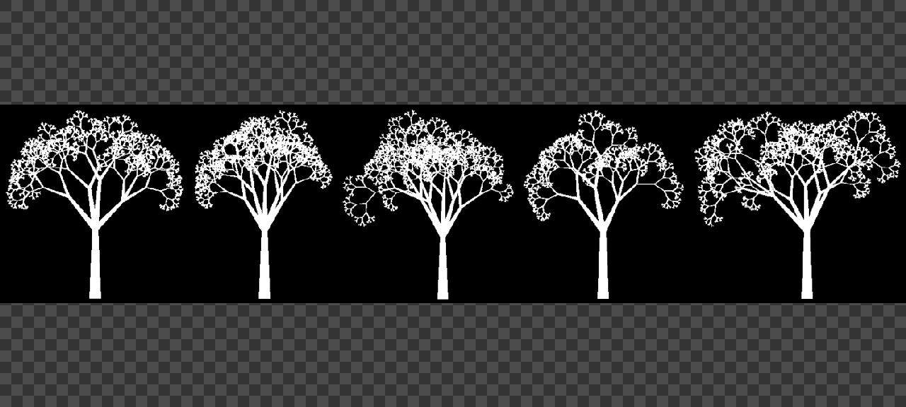
So after playing with code and tweaking it, this is what I get (in 2D only for now):

with the following code:

foo :

  # Build structure of the tree.
  1,1,1,7 => active
  1,1,1,7 => done
  eval "
    const nbp = 512;

    add_branch(__P0,__P1,__level) = (
      ref(__P0,_P0); ref(__P1,_P1); ref(__level,_level);
      _dP = _P1 - _P0;
      _length = norm(_dP);
      _U = unitnorm(_dP);
      _V = [ _U[1],-_U[0] ];
      _alpha = u(0.35,0.85);
      _beta = u(0.15*_level^0.5)*(u<0.5?-1:1);
      _Pc = _P0 + _length*(_alpha*_U + _beta*_V);
      da_push(#$active,[ _P0,_Pc,_P1,_level] );
    );

    # Generate trunk
    add_branch([0.5,1],[0.5 + 0.025*g,0.45],1);

    # Recursively add sub-branches.
    while (siz = da_size(#$active),
      ind = v(siz - 1);
      B = I[#$active,ind];
      level = B[6];

      level<4?(
        P0 = [ B[0],B[1] ];
        Pc = [ B[2],B[3] ];
        P1 = [ B[4],B[5] ];
        xs = resize([ P0[0],Pc[0],P1[0] ],nbp,5);
        ys = resize([ P0[1],Pc[1],P1[1] ],nbp,5);
        length = norm(P1 - P0);

        repeat (int(v(10,20)/level),
          nind = v(nbp/(4 + level),nbp - 1);
          nP0 = [ xs[nind],ys[nind] ];

          ang = atan2(ys[nind -1] - nP0[1],xs[nind - 1] - nP0[0]);

          twist = u(pi/6,pi/3);

          nang = ang + pi/2 + (u<0.5?twist:pi - twist);

          nU = [ cos(ang),sin(ang) ];
          nV = [ cos(nang),sin(nang) ];
          nlength = u(0.1,0.5)*length;
          nP1 = nP0 + nlength*nV;
          add_branch(nP0,nP1,level + 1);
        );
      );

      da_push(#$done,B);
      da_remove(#$active,ind);
    );
    da_freeze(#$done)"
  rm[active]

  # Draw the tree.
  500,500 => canvas
  eval[done] ">
    const nbp = 512;
    B = I;
    P0 = [ B[0],B[1] ];
    Pc = [ B[2],B[3] ];
    P1 = [ B[4],B[5] ];
    xs = resize([ P0[0],Pc[0],P1[0] ],nbp,5)*(w#$canvas - 1);
    ys = resize([ P0[1],Pc[1],P1[1] ],nbp,5)*(h#$canvas - 1);

    ox = oy = -1;
    repeat (nbp,k,
      x = xs[k]; y = ys[k];
      x!=ox || y!=oy?(i(#$canvas,xs[k],ys[k])+=1);
      ox = x;
      oy = y;
    )"
  rm[done]
  normalize_local. , pow. 0.25 autocrop. frame. xy,10,0 n. 0,255

All those are drawn as series of 2D splines, so extending this algorithm to 3D should be straightforward (hopefully). And the structure we get starts to look like trees at least :slight_smile:

But before going into 3D, I’m going to try and thicken things up a bit, because at the moment they look more like little plants than trees. With a thick, fat, trunk, it should look better…

Stay tuned!

2 Likes

And i think you should keep this version as a little plants generator since they look good i think.


res 1500,1500 + dilate_circ 5 + a quick color gradient

I wouldn’t my adding some of these in my grass script.

PS: Any reason why autocrop fails at 1100x1100px and above?
At least it happens to me with this script.

1 Like

Back to straight lines

I was a little annoyed that my trees looked more like little plants than trees, so I went back to the algorithm I’d used in my “Rendering / Tree” filter, which was already in the G’MIC-Qt plug-in. And I decided to rewrite something similar, with the idea of being able to do something simple that I could easily extend for 3D volume images.

So I put the splines aside (temporarily), to keep only straight segments to render the branches, but integrating from the start the idea that these branches had to have a thickness.
And instead of grafting branches randomly onto existing ones, I added them at the ends.

So in the end, a lot of simplifications made, but at least the result looks more like trees than before! Here is how it looks now:

Now that I have this (correct enough) basis, I’ll try first to replace segments back with splines (yes, I’m stubborn!) and then, if everything looks good, start the extension to the 3D world!
In short, I’m not there yet!

Here is the current version of the code:

foo :
  500,500 => canvas
  1,1,1,5 => list
  eval "
    const wc = w#$canvas;
    const hc = h#$canvas;

    add_branch(__P0,__P1,_level) = (
      ref(__P0,_P0); ref(__P1,_P1);

      # Add branch in active list.
      da_push(#$list,[ _P0,_P1,_level ]);

      # Draw branch on canvas.
      _dP = _P1 - _P0;
      _U = unitnorm(_dP);
      _V = [ -_U[1],_U[0] ];
      _R0 = max(1,20*2^-_level);
      _R1 = _R0/2;
      _Ppp = _P0 - _R0*_V;
      _Pnp = _P0 + _R0*_V;
      _Ppn = _P1 - _R1*_V;
      _Pnn = _P1 + _R1*_V;
       polygon(#$canvas,4,_Ppp,_Pnp,_Pnn,_Ppn,1,1);
    );

    # Add initial trunk.
    add_branch([wc/2,hc - 1],[wc/2,0.75*hc],1);

    # Generate sub-branches recursively.
    while (siz = da_size(#$list),
      B = da_pop(#$list);

      P0 = B[0,2];
      P1 = B[2,2];
      level = B[4];

      level<10?( # Add sub-branches
        levelp1 = level + 1;
        dP = P1 - P0;
        U = unitnorm(dP);
        L = norm(dP);

        nb_branches = max(2,v(4,8)*1.5^-level);
        repeat (nb_branches,k,
          ang = lerp(u(-45,-30),u(30,45),k/(nb_branches - 1));
          nU = rot(ang°)*U;
          nL = u(0.5,0.75)*L;

          add_branch(P1,P1 + nL*nU,levelp1);
        );
      );
    )"
  k[canvas] autocrop frame xy,10,0

¿Por que no los dos?

Why not both? Both is good.

Sure, but the title of my OP is “Building 3D trees” :slight_smile:
And this time, my goal is not really to create a new filter, but rather a G’MIC script that can export 3D trees as .obj files.

Bend those branches!

So I tried to replace the perfectly straight branches I’d generated in my previous post with curved branches using splines, but keeping the branch thickness.

And that’s where the serious problems start. Drawing a spline of a certain thickness, with a radius that also varies locally, turns out to be quite painful to do.

The idea of just drawing, at each point of the spline, a segment oriented along the normal vector local to that point may seem like a good idea, but in practice images live in a discrete world, and doing this generates lots of holes all over the interior of the branches.
(many of the pixels you’d like to set are actually never crossed by the hundreds of segments you draw, as if they were deliberately avoiding them :slight_smile: ).

I’ve tried several different strategies to solve this problem, and the only one that really works is to draw a thick spline as a polygon, so this involves keeping a list of all the points on the edges of the thick spline to be drawn.

I could say “OK, let’s do it this way”, but I’m keeping in mind that my little algorithm is going to enter the 3D volumetric world in the near future, and that it’s going to get pretty damn complicated to draw thick 3D splines in a volume image, if I have to do discrete volume mesh filling.

So never mind, I’ve stuck to the idea of drawing segments oriented along the normal at each point, and filling in the gaps as I can:

Here’s what it looks like, with different recursion levels:

It’s not perfect, as a few holes remain, but I’m limiting the damage in this way, and the current algorithm should remain relatively easy to extend into 3D.

And at the very end, I’m going to smooth the volumetric image anyway, before applying marching cubes to obtain the 3D mesh. So this final smoothing should also help remove the few remaining holes! Let’s hope so!

(I’ve spoken to a number of colleagues at the lab who specialize in discrete geometry, and they confirm that this is not an easy problem to solve! It’s good to have specialists on hand :slight_smile: ).

My current code:

tree : check "isint(${1=6},1)"
  nb_levels=$1

  500,500 => canvas
  1,1,1,5 => list
  eval "
    const nbp = 512;
    const wc = w#$canvas;
    const hc = h#$canvas;

    add_branch(__P0,__P1,_level) = (
      ref(__P0,_P0); ref(__P1,_P1);

      # Add branch in active list.
      da_push(#$list,[ _P0,_P1,_level ]);

      # Draw branch on canvas.
      _dP = _P1 - _P0;
      _L = norm(_dP);
      _U = unitnorm(_dP);
      _V = [ -_U[1],_U[0] ];

      _Pc = _P0 + u(_L/3,2*_L/3)*_U + u(_L/4)*(u<0.5?-1:1)*_V;
      _xs = resize([ _P0[0],_Pc[0],_P1[0] ],nbp,5);
      _ys = resize([ _P0[1],_Pc[1],_P1[1] ],nbp,5);
      _R0 = max(1,20*2^-_level);
      _R1 = _R0/2;

      _oP = [ -1,-1 ];
      repeat(nbp,k,
        _P = [ _xs[k],_ys[k] ];
        _Pi = round(_P);
        _R = lerp(_R0,_R1,k/(nbp-1));
        k?(_U = unitnorm(_P - _oP)):(_U = unitnorm([ _xs[1],_ys[1] ] - _P));
        _V = [ -_U[1],_U[0] ];
        _Pl = _P - _R*_V;
        _Pr = _P + _R*_V;
        polygon(#$canvas,2,round(_Pl),round(_Pr),1,1);
        _oP = _P;
      );

    );

    # Add initial trunk.
    add_branch([wc/2,hc - 1],[wc/2,0.75*hc],1);

    # Generate sub-branches recursively.
    while (siz = da_size(#$list),
      B = da_pop(#$list);

      P0 = B[0,2];
      P1 = B[2,2];
      level = B[4];

      level<$nb_levels?( # Add sub-branches
        levelp1 = level + 1;
        dP = P1 - P0;
        U = unitnorm(dP);
        L = norm(dP);

        nb_branches = max(2,v(4,8)*1.5^-level);
        repeat (nb_branches,k,
          ang = lerp(u(-45,-30),u(30,45),k/(nb_branches - 1));
          nU = rot(ang°)*U;
          nL = u(0.5,0.75)*L;

          add_branch(P1,P1 + nL*nU,levelp1);
        );
      );
    )"
  k[canvas] autocrop frame xy,10,0
  f. "const boundary = 1; !i && sum(crop(x-1,y-1,3,3))>6?1:i"

Stay tuned!

Entering the 3D world

As expected, the conversion of my previous algorithm to the 3D world wasn’t much complicated to set up (at least for a first version, which can be of course improved).

I now plot my splines in a 3D volumetric image, and to generate a thickness at each point of the spline, I plot lot of radial segments that make up the disk orthogonal to the spline axis.
I had to write a small code for plotting discrete segments in 3D (rather than using polygon() as I did in 2D), but with G’MIC’s mathematical expression evaluator, it’s easy enough (4 lines of code :slight_smile: ).

Here’s a 3D rendering of the tree shape I get right now:
anim_tree3d-ezgif.com-optimize

I think I still need to rework a bit the way I find the 3D directions of the new branches I’m creating, and a couple of other details to work out, but now it’s starting to look like a 3D tree!

I think I’ve underestimated a bit the difficulty of the task when I took on this challenge.
That’s good, it’s humbling :slight_smile: And I’ve learned a lot of new things in the process!

Here’s my current code that generates the volumetric image:

tree : check "isint(${1=6},1)"
  nb_levels=$1

  500,500,500 => canvas
  1,1,1,7 => list
  eval "
    const nbp = 512;
    const nba = 32;
    const wc = w#$canvas;
    const hc = h#$canvas;
    const dc = d#$canvas;

    add_branch(__P0,__P1,_level) = (
      ref(__P0,_P0); ref(__P1,_P1);

      # Add branch in active list.
      da_push(#$list,[ _P0,_P1,_level ]);

      # Draw branch on canvas.
      _dP = _P1 - _P0;
      _L = norm(_dP);
      _U = unitnorm(_dP);
      _V = unitnorm(cross(_U,[ g,g,g ]));

      _Pc = _P0 + u(_L/3,2*_L/3)*_U + u(_L/4)*(u<0.5?-1:1)*_V;
      _xs = resize([ _P0[0],_Pc[0],_P1[0] ],nbp,5);
      _ys = resize([ _P0[1],_Pc[1],_P1[1] ],nbp,5);
      _zs = resize([ _P0[2],_Pc[2],_P1[2] ],nbp,5);
      _R0 = max(1,20*2^-(_level - 1));
      _R1 = _R0/2;

      _oP = [ -1,-1,-1 ];
      repeat(nbp,k,
        _P = [ _xs[k],_ys[k],_zs[k] ];
        _R = lerp(_R0,_R1,k/(nbp-1));
        k?(_U = unitnorm(_P - _oP)):(_U = unitnorm([ _xs[1],_ys[1],_zs[1] ] - _P));
        _V = unitnorm(cross(_U,[ g,g,g ]));

        repeat (nba,a,
          ang = lerp(0,180,a/nba)°;
          _W = rot(_U[0],_U[1],_U[2],ang)*_V;
          _Pl = _P - _R*_W;
          _Pr = _P + _R*_W;

          # Draw 3D segment.
          _sn = norm1(_Pr - _Pl);
          repeat (_sn + 1,p,
            _sP = round(lerp(_Pl,_Pr,p/_sn));
            i(#$canvas,_sP[0],_sP[1],_sP[2]) = 1;
          );
        );

        _oP = _P;
      );

    );

    # Add initial trunk.
    add_branch([wc/2,hc - 1,dc/2],[wc/2,0.75*hc,dc/2],1);

    # Generate sub-branches recursively.
    while (siz = da_size(#$list),
      B = da_pop(#$list);

      P0 = B[0,3];
      P1 = B[3,3];
      level = B[6];

      level<$nb_levels?( # Add sub-branches
        levelp1 = level + 1;
        dP = P1 - P0;
        U = unitnorm(dP);
        L = norm(dP);

        nb_branches = max(2,v(4,8)*1.5^-level);
        repeat (nb_branches,k,
          V = unitnorm(cross(_U,[ g,g,g ]));
          nU = unitnorm(U + u(0.5,2)*V);
          nL = u(0.5,0.75)*L;
          add_branch(P1,P1 + nL*nU,levelp1);
        );
      );
    )
  "
  k[canvas]

Then I use command display_voxels3d to view it:

$ gmic tree 8 autocrop 0 frame xyz,10,0 dv3d
1 Like

It looks really good. I can see myself using this to make game assets.

1 Like

Converting to 3D mesh

In the end, I was able to improve the algorithm heuristics for choosing directions and the number of branches, and the result is 3D trees that are now a little more balanced.

And then, to validate all this, I’ve used the isosurface3d command, which uses the marching cubes algorithm to generate a 3D mesh made up of triangles, starting from a slightly smoothed version of the volume image containing the binary 3D tree.

All that remained was to save the mesh in .obj format (Wavefront), and import it back into Blender!

A good idea would probably be first to reduce the number of triangles by using one of the 3D mesh simplification algos included in Blender, as for the moment, these are still rather large objects in terms of the number of triangles (over 500k in the figure above).

Well, I think I’ve finally reached my goal! :sweat_smile:

Of course, there are lots of fun things I could have tried out (adding leaves, for example), but I have to admit that it’s already taken me longer than expected, so I’ll stop here for now.

Here’s the final G’MIC script, to generate a spline-based fractal tree. Feel free to test it, play with it and modify it to suit your needs!

tree3d : check "isint(${1=6},1)"
  nb_levels=$1

  500,500,500 => canvas
  1,1,1,7 => list
  eval "
    const nbp = 256;
    const nba = 128;
    const wc = w#$canvas;
    const hc = h#$canvas;
    const dc = d#$canvas;

    add_branch(__P0,__P1,_level) = (
      ref(__P0,_P0); ref(__P1,_P1);

      # Add branch in active list.
      da_push(#$list,[ _P0,_P1,_level ]);

      # Draw branch on canvas.
      _dP = _P1 - _P0;
      _L = norm(_dP);
      _U = unitnorm(_dP);
      _V = unitnorm(cross(_U,[ g,g,g ]));

      _Pc = _P0 + u(_L/3,2*_L/3)*_U + u(_L/4)*(u<0.5?-1:1)*_V;
      _xs = resize([ _P0[0],_Pc[0],_P1[0] ],nbp,5);
      _ys = resize([ _P0[1],_Pc[1],_P1[1] ],nbp,5);
      _zs = resize([ _P0[2],_Pc[2],_P1[2] ],nbp,5);
      _R0 = max(1,20*2^-_level);
      _R1 = _R0/2;

      _oP = [ -1,-1,-1 ];
      repeat(nbp,k,
        _P = [ _xs[k],_ys[k],_zs[k] ];
        _R = lerp(_R0,_R1,k/(nbp-1));
        k?(_U = unitnorm(_P - _oP)):(_U = unitnorm([ _xs[1],_ys[1],_zs[1] ] - _P));
        _V = unitnorm(cross(_U,[ g,g,g ]));

        # Draw disk orthogonal to spline axis.
        _nba = max(16,nba*2^-_level);
        repeat (_nba,a,
          ang = lerp(0,180,a/nba)°;
          _W = rot(_U[0],_U[1],_U[2],ang)*_V;
          _Pl = _P - _R*_W;
          _Pr = _P + _R*_W;

          # Draw 3D segment.
          _sn = norm1(_Pr - _Pl);
          repeat (_sn + 1,p,
            _sP = round(lerp(_Pl,_Pr,p/_sn));
            i(#$canvas,_sP[0],_sP[1],_sP[2]) = 1;
          );
        );

        _oP = _P;
      );

    );

    # Add initial trunk.
    add_branch([wc/2,hc - 1,dc/2],[wc/2,0.75*hc,dc/2],0);

    # Generate sub-branches recursively.
    while (siz = da_size(#$list),
      B = da_pop(#$list);

      P0 = B[0,3];
      P1 = B[3,3];
      level = B[6];

      level<$nb_levels?( # Add sub-branches
        levelp1 = level + 1;
        dP = P1 - P0;
        U = unitnorm(dP);
        L = norm(dP);

        nb_branches = max(2,v(2,5)*1.15^-level);
        V0 = unitnorm(cross(_U,[ g,g,g ]));

        repeat (nb_branches,k,
          V = rot(U,deg2rad(360*k/nb_branches + 5*g))*V0;
          nU = unitnorm(U + u(0.75,1)*V);
          nL = u(0.5,0.75)*L;
          add_branch(P1,P1 + nL*nU,levelp1);
        );
      );
    )


  "
  k[canvas]

  # Convert to 3D mesh.
  autocrop 0 b 1.25 isosurface3d 0.15 rv3d
1 Like