Got an image problem ? Go see the image doctor.

anon41087856 · October 18, 2019, 12:34am

#StoryTime

Some of you know I started to dive into the image processing dev side a few years ago, with blind deconvolution. I can’t believe this was already 2 years and 25.628 lines of code (in darktable’s core) ago.

2.5 years ago, I saw an advertisement on Instagram about some software (can’t remember the name now) that did blind deconvolution for image sharpening. I was at Polytechnique Montréal, in engineering school, studying boring mechanical engineering (school was boring as Hell, not engineering itself), and shooting portraits of people to forget about it. It was a Friday night, my girlfriend was already sleeping, I had nothing better to do than scouting Google Scholar about it.

Blind deconvolution is the process by which you try to estimate the blurring function of the lens (Point Spread Function, or PSF for geeks) while you actually deblur the picture. The drill is as follow:

infer a rough PSF,
while you are not happy about the result and your computer didn’t overheat :
- sharpen the picture a little bit by reverting the estimated PSF,
- refine the PSF estimation by comparing the sharpened picture with the original picture.

That’s basically supervised machine learning. I was not prepared for that. In French, we have a saying : « Bon à rien, prêt à tout » (good for nothing, ready for everything). That’s me.

That lead to some painfully slow Python prototype, that eventually became an half-working darktable’s module, thanks to @Edgardo_Hoszowski . But still, I wasn’t happy about it : the runtime was beyond usable, the results quality was random, and more importantly, the deblurring algo didn’t care for the already sharp parts of the pictures.

14 months ago, after I spent 1.5 year repeating to myself “I will have to learn the C programming language to start contributing in darktable at some point”, I decided I couldn’t continue to be a loser with blank dreams, so I stopped sleeping, learned C, SSE2 intrinsics and OpenCL altogether, and 2 months later, Filmic v1 was born. 4 months later, I had 13.207 lines of code merged in darktable’s core (these 13.000 lines were mostly bugs, and code quality doesn’t measure in code volume, but just let me brag, okay ?).

Anyway, the point is I didn’t give up on deconvolution, and as I developed the tone equalizer and started playing with guided filters, I got another idea : why not replace the Richardson-Lucy-like deconvolution scheme with an iterative unsharp-masking based on guided filters ? That would ignore already-sharp edges (no over-sharpening) and halos altogether. How nice ?

Well, that’s done.

Before (credit: BPN Photo - 50 mm F/1.4):

After:

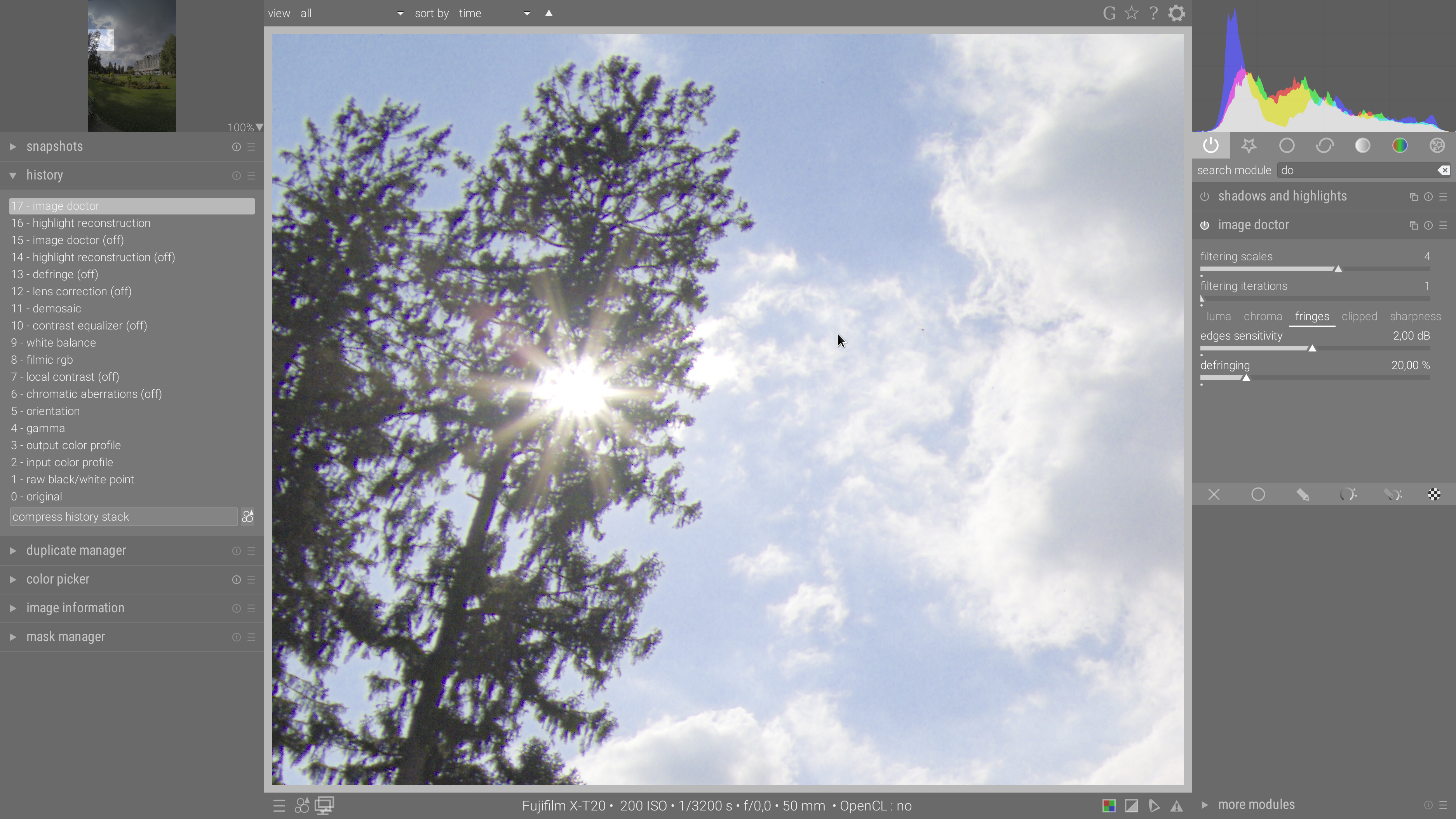
I’m working on another darktable module that would reconstruct any damaged part of a picture: image doctor. The goal is to perform a multi-scale denoising, sharpening, and fringes removal at once, using guided filters and inter-channel correlation assumptions.

Try it (crazy slow, unoptimized, R&D material, backup your database, etc.):

How does it work ?

Chroma denoising

On an RGB picture, if you compute the R-G, B-G and G-R-B layers, you will find out that they are pretty much piece-wise smooth, meaning you get smooth surfaces inside of edges. Luckily, the guided filter provide an edge-aware surface blur, meaning it can stop at edges and blur inside. Note that we don’t aim here at fully denoising the picture (which is usually ugly and unnatural), but rather at making the noise more pleasing (finer and more even). Also, we won’t care about the PSNR as most academic papers do, because they try to denoise synthetic blur added on top of the IMAX or Kodak (scanned film) sRGB image dataset, and we aim at denoising any raw linear image in whatever stupid ill-behaved RGB space your camera records in, in a fashion that let you print satisfying pictures.

Let us denote \mathscr{G}(image, guide) the guided filter. The chroma denoising iteratively performs:

\begin{equation} B_i = (1 - \alpha) B_{i - 1} + \alpha (G_{i - 1} - \mathscr{G}(B_{i - 1} - G_{i - 1}, B_{i - 1} -G_{i - 1}) ) \\ R_i = (1 - \alpha) R_{i - 1} + \alpha (G_{i - 1} - \mathscr{G}(R_{i - 1} - G_{i - 1}, R_{i - 1} - G_{i - 1}) )\\ G_i = (1 - \alpha) G_{i - 1} + \alpha (R_{i - 1} - \mathscr{G}(G_{i - 1} - R_{i - 1}, G_{i - 1} - R_{i - 1}) + B_{i - 1} - \mathscr{G}(G_{i - 1} - B_{i - 1}, G_{i - 1} - B_{i - 1})) \end{equation}

where i it the current iteration and \alpha is a user-set strength parameter for the denoising (which falls-back to a simple alpha blending, very suitable with the linear nature of the guided filter output). Note that the guided filter is used here as a simple surface blur.

Before (extended 64508 ISO, under-exposed by 2.86 EV, on Nikon D500 — talk about real-life example - credit mimi85):

After:

Notice that this approach is not enough to fully denoise an image, but it is a very nice complement to @hanatos and @rawfiner work on the non-local means denoising, and might allow to go softer on this module (and get more sharpness) while still getting good-looking photographic results (if anyone here ever shot Ilford Delta 3200, you know grain is not always evil).

Defringing

I got some inspiration from iterative guided upsampling by residual interpolation for raw demosaicing. Most defringing algos do an edge detection (with a Laplacian filter or similar, which is essentially a second-order derivative approximation) and desaturate those edges in Lab or HSV. However, they don’t make an exception for valid sharp and saturated edges, like lipstick or road signs in Europe, so witness the grey-edged lipstick on your models. Sad…

Fringes (chromatic aberrations) happen when R, B, and G channels are decorrelated due to the wavelength-dependent refraction indice of glass. Usually, G is centered, while B is on the inside of the picture and R on the outside. The goal is then to squeeze R and B toward G to get a real sharp edge.

The algorithm for defringing is as follow:

Guide each channel with G and compute the residual high frequency:

\begin{equation} HF_B = B - \mathscr{G}(B, G) \\ HF_R = R - \mathscr{G}(R, G) \\ HF_G = G - \mathscr{G}(G, G) \end{equation}

Guide R and B high frequencies with G high frequency:

\begin{equation} \Delta_B = \mathscr{G}(HF_B, HF_G) \\ \Delta_R = \mathscr{G}(HF_R, HF_G) \\ \Delta_G = \mathscr{G}(HF_G, HF_G) \end{equation}

Correct each RGB channel with that:

\begin{equation} R = R + \alpha \Delta_R \\ B = B + \alpha \Delta_B \\ G = G + \alpha \Delta_G \\ \end{equation}

with \alpha a user-set strength parameter, usually between 0.05 and 0.1.

Before (credit : @rawfiner):

After:

Meanwhile, check that we didn’t mess-up the red flowers:

Before:

After:

We are good.

Sharpening

Well, it’s an iterative unsharp mask with a box window increasing by 2 at each iteration. Nothing new here, except we use a guided filter as an edge-aware blurring operator to avoid gradient reversal. See example on the 2 first images in this post.

Inpainting

I have been investigating the possibility to add inpating based on anisotropic heat diffusion to recover blown highlights along. It’s fully implemented but I don’t reproduce the results of the paper and it produces bad chromatic aberrations. Maybe I’m just a moron and I got it wrong, maybe the examples they show are carefully curated (and none of them are RGB anyway), maybe both. We will see.

FAQ

Will this be included in darktable 3.0 ?

No.

Will you quit horsing around and fix filmic RGB and UI bugs for darktable 3.0 release ?

Yes, I promise.

Is darktable your full-time job ?

Yes, and you can help me help you. Sorry to beg, but you know… rent and health insurance… Basically, R&D like that or like the tone equalizer takes a lot of time, not just programing, but also testing and tweaking the algo, refining user-interaction, getting feedback and remote-fixing weird Windows/Mac bugs that don’t reproduce on Linux.

What beer do you like ?

Christmas beers will start to show up soon

paperdigits · October 18, 2019, 12:52am

Well holy shit, that’s cool.

afre · October 18, 2019, 1:01am

Very cool. So who is the doctor?

I have always been wrestling with the same issues as you have been but you are 1000 years ahead of me. And yes, inpainting is also the subject that I am struggling with the most. The results are so unreliable.

anon41087856 · October 18, 2019, 1:11am

The doctor is in the software ^^.

Definitely.

hanatos · October 18, 2019, 7:35am

this looks very awesome. essentially you’re saying you can do a better edge-aware wavelet transform with iterated guided filters, using green as guide? sounds risky for very noisy images, but your example seems to prove otherwise.

this reminds me i need to implement the fully generic guided filter in fast.

anon41087856 · October 18, 2019, 7:47am

Exactly, but the approach is a bit different since:

I don’t actually decompose the image into frequency “bands”, but apply the filter again and again in a serialized way, on top of itself, and varying the window size,
borrowing to the guided upsampling paper, and confirmed in practice, varying the window size from fine to coarse is better than from coarse to fine (which is the classic pyramidal approach).

For noise reduction, the guided filter falls back to a local patch-wise variance estimation, which I believe could be used to auto-profile the noise reduction with a single image. The theory is yet to write formally.

anon41087856 · December 2, 2019, 1:06am

@Carmelo_DrRaw I might have found a way for the enhanced USM to limit it to the actual depth of field, and then increase it or reduce it.

The principle is to blend the result of the band-pass USM with an alpha layer such that:

out(i, j) = in (i, j) + \alpha(i, j) × strength × BP(i, j),

where BP = 2 HF_{low} - HF_{high} (I know you use BP = HF_{low} - HF_{high} but I find the cut-off too harsh), and HF = image - LF

The alpha mask is build by guiding \dfrac{HF_{high} + HF_{low}}{||LF_{high} + LF_{low}||_2} with BP. You can tweak the formula to allow the user to rescale the depth of field map:

\dfrac{HF_{high} + HF_{low}}{||LF_{high} + LF_{low}||_2} + (1 - DOF)

With DOF > 1, the depth of field is made shorter (more blur), and the other way around. Notice that the alpha mask is not a standard premultiplied alpha. Also, you an apply this setup iteratively to get an edge-aware sort of blind deconvolution.

This is all a bit hacky and ad-hoc, I need to check the math to verify the sense of what I’m doing, but what do you think so far ?

anon41087856 · December 4, 2019, 2:49am

Ok the above equations didn’t worked as well as I would have liked. I finally choose a simple deconvolution scheme with total variation regularization, and without the band pass filter.

Example with https://discuss.pixls.us/t/playraw-view-on-the-mosel/15099/2:

Before:

After:

Notice how the background has not been deblurred while the foreground is much sharper. Also the transition is very progressive.

Jean-Paul_GAUCHE · December 4, 2019, 8:55pm

Excellent Aurélien.

ari · December 13, 2019, 9:12pm

Outstanding effort! landed here after running into an older Youtube video from Aurelien that discusses the initial deconvolution effort that I thought was discontinued - it’s always really humbling to see amazing contributions coming to DT. This new module is shaping up nicely.
Is it meant to replace sharpen+local contrast or to complement either or both?

anon41087856 · December 17, 2019, 6:02pm

It should replace sharpen to restore optical sharpness, but local contrast is more of a perceptual thing, so it’s not the same.

betazoid · December 21, 2019, 11:54am

Is denoise profile non local faster in this version (or is it because I changed my system)?

T_N_Args · February 5, 2020, 12:54pm

“2.5 years ago, I saw an advertisement on Instagram about some software (can’t remember the name now) that did blind deconvolution for image sharpening.”

Piccure?

I tried it and I struggled with halos on its output, so gave up before long.

Looking forward to where this project ends up.

cheers

anon41087856 · February 5, 2020, 1:03pm

Yep, this one !

GBB29 · February 5, 2020, 2:07pm

Oh, piccure… took forever, did little

Anyway, Aurélian: it seems that guided filters are your leit motif… where can I read something precise but elementary (!!) about what they are and how they work?

anon41087856 · February 5, 2020, 2:11pm

Well, they are quite elegant in their formulation, faster than most filters, and don’t have gradient reversal effects as the bilateral filter does, so…

Here is the base paper:
http://kaiminghe.com/eccv10/

GBB29 · February 5, 2020, 2:41pm

So I read one of Kneyazev’s arxiv papres, on guided operators. Looks cool, but I don’t get where the guiding image comes from… or I can imagine that it’s the original scene referred linear RGB when applying luminosity changes (forgive the imprecision) via something like the tone equalizer. But in blind deconvolution?

(This is not a million km from my work, which sometimes involves blind source separation to detect “signatures” of carcinogens, but tend to be strongly influenced by non-linear effects of the constraints… and the investigators’ prejudices).

anon41087856 · February 5, 2020, 2:54pm

The guiding image can be the image itself (useful to remove blur), or one RGB channel can be used to guide another (useful to remove noise or chromatic aberrations).

The point of guiding the image with itself is to create a surface blur (as in the the tone equalizer). If you subtract the surface blur from the original image, you get an high frequency isolation with a variance thresholding to ignore sharp things. So, when you reapply the high frequency on top of the image (which is the base of the unsharp masking and the deconvolution), you don’t increase the already sharp details (which is responsible for halos). But also, if you repeat that process iteratively and make the blur radius and variance threshold vary along the process, you can remove static blurs as a blind deconvolution would do but without having to estimate the PSF (it’s kind of an implicit PSF). You can’t do that with usual deconvolution, since deconvolving with a wrong PSF will lead to artifacts (and PSF vary in the frame). But because of the variance threshold (and the depth of field mask I add), the guided-filter-based deconvolution is auto-dampened where the surface blur doesn’t match accurately the real blur in the picture, so the artifacts creation is well controlled, plus the implicit PSF is patch-wise, so we account for the lens distortion.

GBB29 · February 5, 2020, 3:36pm

Oh, of course, you’re using (combinations of) RGB components to adjust the other components… which you said, somewhere. Doh.
So as long as there isn’t a peculiar dependence of texture on chroma, it should work… more or less as an expectation-maximisation algorithm.

Otoh, the tone equalizer lives downstream of the channel mixer… which can be used to create monochrome images. So what happens then?

Le mer. 5 févr. 2020 à 15:59, Aurélien Pierre via discuss.pixls.us noreply@discuss.pixls.us a écrit :

anon41087856 · February 5, 2020, 4:05pm

Tone equalizer comes before channel mixer, so everything is fine regarding colour.

Chroma doesn’t mean anything at this stage of the pipe, since we didn’t do chromatic adaptation yet. The CFA broke the spectrum into 3 RGB layers, as far as we are concerned here, we are only dealing with gradient fields and enforcing their patch-wise correlation.